This is one in a series of posts about the Google Technology Stack – PageRank, MapReduce, and so on – based on a lecture series I’m giving in 2008 and 2009. If you’d like to know more about the series, please see the course syllabus. There is a FriendFeed room for the series here.
Today’s post overviews the technologies we’ll be discussing in the course, and introduces the basics of the PageRank algorithm.
Introduction to PageRank
Introduction to this course
Here’s a cartoon picture of the technologies powering Google: 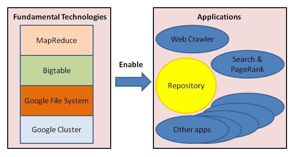
The picture is not entirely accurate – a point I’ll return to shortly – but it is a good starting point for thinking about what technology could power a company that aims to “organize the world’s information and make it universally accessible and useful”. On the left-hand side of the picture is a stack of fundamental technologies that let Google gather and process enormous quantities of data. To give you an idea of the scale Google works at, in a recent test Google sorted 1 petabyte of data in 6 hours, using a cluster of 4,000 computers. Each day, Google processes more than twenty petabytes of data. The size of the Google cluster doesn’t seem to be public knowledge, but typical estimates place it at several hundred thousand machines, and Google engineers are thinking ahead to a time when the cluster will contain on the order of ten million machines.
On the right-hand side of the picture are the many applications enabled by the fundamental technology stack, including Google’s famous search engine. Also included on the right-hand side is Google’s repository of data, a structured in-house copy of much of the world’s information, including a considerable fraction of the web. The combination of this repository and their other infrastructure provides Google with a proprietary internal platform for innovation that’s matched by no other company.
There’s a caveat to keep in mind here and throughout these lectures: I have never worked at Google. I have friends and acquaintances who work at Google, but we’ve never discussed their work in any depth. The picture above is a caricature, based in part on what Google has published, and in part on my guesses about what’s plausible. You shouldn’t take it seriously as a literal description of what’s going on inside Google. On the other hand, I think the picture shows a pretty plausible core architecture for a large web company. It’s this picture we’ll use as the basis for the lectures, although we won’t discuss all the elements in the picture. In particular, we won’t discuss the actual physical cluster – all the machines, the power systems, the physical network, the cabling, and so on.
Let me digress briefly to clarify a terminological point: I’ve been using the term “cluster” in two ways, to mean both the entire base of machines available to Google, as well as smaller sub-clusters hived off the main cluster and used to run specific jobs, like the 4,000 machines used to sort a petabyte. If you keep the distinction in mind, it should be clear from context which is meant.
Aside from the actual physical cluster, we will discuss all the other technologies pictured above in the fundamental technology stack. Let’s quickly run through what’s in that stack. The Google File System is a simple way of accessing enormous amounts of data spread across a large cluster of machines. It acts as a virtual file system that makes the cluster look to developers more like a single machine, and eliminates the need for developers to think about details like what happens when a machine fails. Bigtable is a simple database system that builds on the Google File System, allowing developers to ignore many of the underlying details of the cluster, and just concentrate on getting things done. MapReduce is a powerful programming model for processing and generating very large data sets on large clusters. MapReduce enables developers to code and run simple but large parallel jobs in minutes, instead of days. More than ten thousand distinct MapReduce programs have been implemented at Google, and roughly one hundred thousand MapReduce jobs are executed on Google’s cluster each day.
What we’ll do in the remainder of this lecture and in the next couple of lectures is study the PageRank algorithm which is at the heart of Google’s search engine. Having looked at the most famous application of Google’s technology, we’ll then back up and return to the fundamental technology stack which makes applications like PageRank possible.
Examples
- (Your everyday Google supercomputer) Suppose Google serves 100 million search queries per day, taking an average of approximately one third of a second to process each uncached query, and that approximately one third of the queries are uncached. Suppose furthermore that 200,000 machines are involved in computing the results of the uncached queries. These numbers are, needless to say, rough estimates.
Using these assumptions, there are approximately 30 million uncached queries per day, and approximately 300,000 query periods, since there are about 100 thousand seconds in a day, and each uncached query takes one third of a second. Thus, on average approximately 100 queries are being performed on the cluster at any given time. This means that a single query harnesses the computational equivalent of approximately 2,000 machines. Every time you use Google for an unusual query, you’re using a supercomputer, albeit one with an exceptionally well-designed user interface!
Exercises
- How realistic do you think the assumptions made in the last example are? Issues worth thinking about include load variability during the day, the fraction of uncached queries, variability in the complexity of different queries, and what fraction of the total cluster it makes business and technical sense to be using on search, versus other applications.
Basic Description of PageRank
What does it mean for a given webpage to be important? Perhaps the most obvious algorithmic way of assessing the importance of a page is to count the number of links to that page. Unfortunately, it’s easy for webpage creators to manipulate this number, and so it’s an unreliable way of assessing page importance. PageRank was introduced as a more reliable way of algorithmically assessing the importance of a webpage.
To understand how PageRank is defined, imagine a websurfer browsing some page on the web. A simple model of surfing behaviour might involve choosing one of the following two actions. Either the websurfer:
- Follows a random link from the page they’re currently on; or
- Decides they’re bored, and “teleports” to a completely random page elsewhere on the web.
Furthermore, the websurfer chooses to do the first action with probability [tex]s[/tex], and the second with probability [tex]t = 1-s[/tex]. If they repeat this random browsing behaviour enough times, it turns out that the probability that they’re on a given webpage [tex]w[/tex] eventually converges to a steady value, [tex]q(w)[/tex]. This probability [tex]q(w)[/tex] is the PageRank for the page [tex]w[/tex].
Intuitively, it should be plausible that the bigger the PageRank [tex]q(w)[/tex] is for a page, the more important that page is. This is for two reasons. First, all other things being equal, the more links there are to a page, the more likely our crazy websurfer is to land on that page, and the higher the PageRank. Second, suppose we consider a very popular page, like, say, www.cnn.com. According to the first reason, just given, this page is likely to have a high PageRank. It follows that any page linked to off www.cnn.com will automatically obtain a pretty high PageRank, because the websurfer is likely to land there coming off the www.cnn.com page. This matches our intuition well: important pages are typically those most likely to be linked to by other important pages.
This intuitive argument isn’t perfect. We’ll see later that there are tricks that can be used to build “link farms” which give spam webpages high PageRanks. If such link farms became too common, then the most important pages on the web, as measured by PageRank, would all be spam pages. The argument in the last paragraph would then be turned upside down: the way to get a high PageRank would be to be linked to by one of those pages, not by a page like www.cnn.com! The spammers would have won.
One aspect of PageRank that is somewhat puzzling upon a first encounter is the teleportation step. One justification for including teleportation is the possibility of our crazy websurfer being led up the garden path, into cliquish collections of pages that only link among themselves. If that happens, our crazy websurfer would get stuck within that clique. The possibility of teleporting solves this garden path problem.
We haven’t yet discussed how the probabilities [tex]s[/tex] and [tex]t[/tex] are set. In the original paper on PageRank, the authors choose [tex]s = 0.85[/tex] and [tex]t = 0.15[/tex]. Intuitively, this seems reasonable – it means that most of the time we are randomly following links, and only occasionally teleporting out, to prevent getting stuck within cliques. This choice for [tex]s[/tex] and [tex]t[/tex] can also be related to the speed at which PageRank can be computed. We’ll see later that by increasing the teleportation probability [tex]t[/tex], we can speed up the computation of PageRank. However, we don’t want to dial [tex]t[/tex] all the way up to the maximum possible value [tex]t=1[/tex], for to do so would mean that we lost all the information about page importance contained in the link structure of the web. Instead, it is best to choose an intermediate value, which ensures that PageRank both strongly reflects the link structure, and can be computed relatively quickly. The values [tex]s = 0.85[/tex] and [tex]t = 0.15[/tex] fulfill both these criteria, and so we’ll use those in our examples.
Variations on PageRank
There are many variations on PageRank, too many to discuss in detail here. We will, however, describe two of the most common variations.
Dangling pages: The first variation has to do with dangling pages, that is, pages that have links coming into them, but no links coming out. If you think about our earlier description of the crazy websurfer, the description doesn’t specify how the websurfer should behave if they come to a dangling page.
There are many approaches we could take to extending PageRank to dangling pages. Perhaps the simplest is to eliminate dangling pages (and links to dangling pages) from the description of the web, and to only compute PageRank for non-dangling pages. This approach has the virtue of simplicity, but it also runs the risk of eliminating some important pages from consideration by the PageRank algorithm. A second approach is to modify PageRank so that if our random websurfer comes to a dangling webpage, they apply the teleportation step with probability one. In terms of our crazy websurfer model, this is equivalent to modifying the link structure of the web so the dangling page links to every single page on the web.
Now, for the purposes of subsequent discussion it’s not going to matter much which of these two approaches is used. To make things concrete, we’ll assume that the second approach is what’s used. But both approaches are effectively equivalent to modifying the link structure of the web in some way, and so everything we say will apply to both approaches, and also to many other natural ways of tackling the problem of dangling pages.
Personalizing PageRank: The second variation of PageRank we’ll consider involves a modification of the teleportation step. Instead of teleporting to a randomly chosen page, suppose our crazy websurfer teleports to a page randomly chosen from some fixed distribution [tex]P = P(w)[/tex] over all webpages. This modified teleportation step can potentially be used to personalize PageRank, e.g., by choosing the distribution [tex]P[/tex] to be peaked at the user’s homepage, or on some subset of pages that the user is known to like a great deal. Of course, the original PageRank algorithm is a special case of this one, obtained by choosing [tex]P[/tex] to be a uniform distribution over webpages.
Matrix description of the websurfer
Let’s recast the behaviour of our crazy websurfer in a more compact matrix description. Suppose for convenience that we number webpages from [tex]1,\ldots,N[/tex]. We’ll imagine for now that the number of webpages and the links between them are fixed. Furthermore, suppose the initial location of the crazy websurfer is described by an [tex]N[/tex]-dimensional probability distribution [tex]p = (p_1,\ldots,p_N)[/tex]. The location after one step will be described by the probability distribution [tex]Mp[/tex] where we regard [tex]p[/tex] as an [tex]N[/tex]-dimensional vectors, and where [tex]M[/tex] is an [tex]N \times N[/tex] matrix given by
[tex] M = s G + t E. [/tex]
Here, [tex]G[/tex] is a matrix which represents the random link-following behaviour. In particular, the [tex]k[/tex]’th column of [tex]G[/tex] has entries describing the probabilities of going to other pages from page [tex]k[/tex]. If [tex]\#(k)[/tex] is the number of links outbound from page [tex]k[/tex], then those probabilities are [tex]1/\#(k)[/tex]:
[tex] G_{jk} = \left\{ \begin{array}{l} \frac{1}{\#(k)} \mbox{ if page } k \mbox{ links to page } j \\ 0 \mbox{ if page } k \mbox{ does not link to page } j. \end{array} \right. [/tex]
If page [tex]k[/tex] is a dangling page, then we imagine that it has links to every page on the web, and so [tex]\#(k) = N[/tex], and [tex]G_{jk} = 1/N[/tex] for all [tex]j[/tex].
The matrix [tex]E[/tex] describes the teleportation step. In the case of the original PageRank algorithm, [tex]E_{jk} = 1/N[/tex], the probability of teleporting from page [tex]k[/tex] to page [tex]j[/tex]. In the case of personalized PageRank, [tex]E[/tex] consists of repeated columns containing the personalization distribution, [tex]P[/tex], i.e., [tex]E_{jk} = P_j[/tex]. Note that we use the same notation [tex]E[/tex] regardless of whether we’re working with the original PageRank algorithm, or with the personalized variant.
We pause to note a useful algebraic fact about [tex]E[/tex] that we’ll use repeatedly,
[tex] E v = s(v) P, [/tex]
where [tex]s(v)[/tex] is defined to be the sum of all the entries in [tex]v[/tex]. This equation follows from straightforward manipulations: [tex](Ev)_j = \sum_k E_{jk} v_k = \sum_k P_j v_k = s(v) P_j[/tex].
To people who’ve previously worked with random walks or Markov chains, the matrix-theoretic description of the crazy websurfer’s random walk given above will be familiar. If you’re not comfortable with those tools, though, you should work through the next two exercises, and the example which follows.
Exercises
- Prove that the equation [tex]p \rightarrow Mp[/tex] describes the way the probability distribution changes during a single timestep for the crazy websurfer.
- (Stochastic matrices) Prove that all the entries of [tex]M[/tex] as defined above are non-negative, and that all the columns of [tex]M[/tex] add up to one. Matrices with both these properties are called stochastic matrices, and the equation [tex]p \rightarrow Mp[/tex] with [tex]M[/tex] a stochastic matrix is a general way of describing random walks on a state space.
Examples
- It’s not just the matrix [tex]M[/tex] which is stochastic. The matrices [tex]G[/tex] and [tex]E[/tex] are also stochastic. To see that [tex]G[/tex] is stochastic, just notice that the [tex]j[/tex]th column has [tex]\#(j)[/tex] non-zero entries, all [tex]1/\#(j)[/tex], and so they sum to one. To see that [tex]E[/tex] is stochastic, notice that each column is a probability distribution, and so the entries must be non-negative and sum to one.
Defining PageRank
We gave an informal definition of PageRank above, but let’s now make a more precise definition. It turns out that there are many equivalent ways of doing this. An especially simple way, and the way we’ll go here, is to define the PageRank distribution [tex]q[/tex] as the probability distribution [tex]q[/tex] which is unchanged by the random walk, i.e.,
[tex] q = Mq. [/tex]
This approach to a definition accords with our intuition that the probability distribution of the crazy websurfer gradually settles down to a stable distribution. To show that the definition actually makes sense, and has the properties we desire, we have to show that such a probability distribution (1) exists; (2) is unique; and (3) corresponds to the limiting distribution. We’ll do all these things over the remainder of this section, and in the next section.
To prove existence and uniqueness, first substitute our earlier expression [tex]M = s G + t E[/tex] into the equation [tex]Mq = q[/tex], and rearrange, so we see that [tex]Mq = q[/tex] is equivalent to [tex](I-sG)q = tEq[/tex]. Recall that [tex]Eq = s(q) P[/tex], where [tex]s(q)[/tex] is just the sum of all the entries in the vector [tex]q[/tex]. We’ll eventually see that a [tex]q[/tex] satisfying [tex]Mq = q[/tex] exists and satisfies [tex]s(q) = 1[/tex], as we’d expect for a probability distribution, but for now we make no such assumption. It follows that [tex]Mq = q[/tex] is equivalent to
[tex] (I-sG) q = t s(q) P. [/tex]
The key to analysing the existence and uniqueness of solutions to the equation [tex]Mq = q[/tex] is therefore to understand whether [tex]I-sG[/tex] has an inverse. This is equivalent to asking whether [tex]I-sG[/tex] has any zero eigenvalues, and so, since [tex]G[/tex] is a stochastic matrix, we will need to understand some facts about the eigenvalues of general stochastic matrices. The fact we need turns out to be that all eigenvalues [tex]\lambda[/tex] of stochastic matrices satisfy [tex]|\lambda| \leq 1[/tex]. We could prove this directly, but our overall presentation turns out to be simplified if we take a slight detour.
The detour involves the [tex]l_1[/tex] norm, a norm on vectors defined by:
[tex] \| v \|_1 \equiv \sum_j |v_j|. [/tex]
Exercises
- If you’re not already familiar with the [tex]l_1[/tex] norm, prove that it is, indeed, a norm on vectors, i.e., [tex]\| v\|_1 \geq 0[/tex], with equality if and only if [tex]v = 0[/tex], [tex]\| \alpha v \|_1 = |\alpha| \|v \|_1[/tex] for all scalars [tex]\alpha[/tex], and [tex]\|v + w \|_1 \leq \|v\|_1 + \|w\|_1[/tex].
- (Interpretation of the [tex]l_1[/tex] norm) Suppose [tex]p[/tex] and [tex]q[/tex] are probability distributions over the same sample space. Imagine that Alice flips a fair coin, and depending on the outcome, samples from either the distribution [tex]p[/tex] or [tex]q[/tex]. She then gives the result of her sampling to Bob. Bob’s task is to use this result to make the best possible guess about whether Alice sampled from [tex]p[/tex] or [tex]q[/tex]. Show that his best possible guessing strategy has a correctness probability of [tex] \frac{1+\|p-q\|_1/2}{2}. [/tex]
Proving this formula is a challenging but worthwhile exercise. The formula provides a nice intuitive interpretation of the [tex]l_1[/tex] norm, as determining the probability of Bob being able to distinguish the two probability distributions. Notice that it matches up well with our existing intuitions. For example, when [tex]p = q[/tex], there’s nothing Bob can do to tell which distribution Alice sampled from, and so the best possible strategy for Bob is just to randomly guess, giving a probability [tex]1/2[/tex] of being right. On the other hand, when the distributions [tex]p[/tex] and [tex]q[/tex] don’t overlap, we see that [tex]\|p-q\|_1 = 2[/tex], and so the probability of Bob being able to distinguish them is [tex](1+2/2)/2 = 1[/tex], as we would expect.
We will prove that stochastic matrices can never increase the [tex]l_1[/tex] norm: intuitively, stochastic matrices “smear out” vectors probabilistically, making them shorter, at least in the [tex]l_1[/tex] norm. This intuition is captured in the following statement:
Theorem:[Contractivity of the [tex]l_1[/tex] norm] If [tex]v[/tex] is a vector and [tex]M[/tex] is a stochastic matrix, then [tex]\| Mv \|_1 \leq \|v\|_1[/tex].
Proof: Substituting the definition of the [tex]l_1[/tex] norm gives
[tex] \| M v\|_1 = \sum_j \left| \sum_k M_{jk} v_k \right| \leq \sum_{jk} M_{jk}|v_k|, [/tex]
where we used the inequality [tex]|a+b| \leq |a|+|b|[/tex] and the fact that [tex]|M_{jk}| = M_{jk}[/tex]. Summing over the [tex]j[/tex] index, and using the fact that the column sums of [tex]M[/tex] are one, we get
[tex] \| M v \|_1 \leq \sum_k |v_k| = \|v\|_1, [/tex]
which is the desired result. QED
The theorem gives as a corollary some information about the eigenvalues of stochastic matrices:
Corollary: If [tex]M[/tex] is a stochastic matrix, then all the eigenvalues [tex]\lambda[/tex] of [tex]M[/tex] satisfy [tex]|\lambda| \leq 1[/tex].
We could have proved this corollary directly, using a strategy very similar to the strategy used in the proof of the contractivity theorem above. But it turns out that the contractivity theorem will be independently useful later in studying the computation of PageRank, and so the overall presentation is simplified by doing things this more indirect way.
(By the way, if you’re familiar with the Perron-Frobenius theorem, it’s worth pausing to note that the corollary is part of the Perron-Frobenius theorem.)
Proof: Suppose [tex]v[/tex] is an eigenvector of [tex]M[/tex] with eigenvalue [tex]\lambda[/tex], so [tex]\lambda v = M v[/tex]. Taking the [tex]l_1[/tex] norm of both sides gives [tex]|\lambda| \| v \|_1 = \|Mv\|_1[/tex], and applying the contractivity of the [tex]l_1[/tex] norm gives [tex]|\lambda| \|v\|_1 \leq \|v\|_1[/tex], and so [tex]|\lambda\| \leq 1[/tex]. QED
This corollary can be recast in a form suitable for application to PageRank.
Corollary: If [tex]M[/tex] is a stochastic matrix, then [tex]I-sM[/tex] is invertible for all [tex]s < 1[/tex]. Proof: For a contradiction, let’s assume it’s not invertible, and so [tex](I-sM) v = 0[/tex] for some non-trivial vector [tex]v[/tex]. This is equivalent to [tex]Mv = \frac{1}{s}v[/tex], and so [tex]M[/tex] has an eigenvalue [tex]1/s > 1[/tex], contradicting the previous lemma. QED
This corollary lets us see two things. First, the equation [tex](I-sG)q = ts(q) P[/tex] cannot have a non-trivial solution [tex]q[/tex] if [tex]s(q) = 0[/tex]. It follows that we can restrict our attention to the case when [tex]s(q) \neq 0[/tex]. By rescaling [tex]q \rightarrow q/s(q)[/tex] this means we can assume without loss of generality that [tex]s(q) = 1[/tex]. Thus [tex]Mq = q[/tex] is equivalent to the equation
[tex] q = t (I-sG)^{-1} P. [/tex]
We see from this argument that [tex]q[/tex] exists, and is uniquely defined up to an overall scaling factor. If we rewrite [tex](I-sG)^{-1}[/tex] as [tex]\sum_{j=0}^\infty s^j G^j[/tex], then we get
[tex] q = t\sum_{j=0}^{\infty} s^j G^j P. [/tex]
Because all the entries of [tex]G[/tex] and [tex]P[/tex] are non-negative, so too are the entries of [tex]G^j P[/tex], and so all the entries of [tex]q[/tex] must be non-negative. Since they sum to one, it follows that [tex]q[/tex] is a probability distribution.
Summing up, we have shown that the equation
[tex] q = t (I-sG)^{-1} P [/tex]
defines a probability distribution which is the unique (up to scaling) non-trivial solution to the equation [tex]Mq = q[/tex]. In the next section we’ll show that this distribution is also the limiting distribution for the random walk of our crazy websurfer. Indeed, you can regard this equation as defining PageRank, since it is equivalent to our earlier definition [tex]q = Mq[/tex], but is more explicit. For this reason we’ll sometimes call this equation the PageRank equation.
One advantage of the PageRank equation is that it immediately shows how to compute PageRank on small link sets, using matrix inverses. For example, the following Python code computes PageRank for a simple three-page “web”, with page 1 linking both to itself and page 2; page 2 linking to page 1 and page 3, and page 3 just linking to itself. Here’s the code:
from numpy import * # imports numerical Python (numpy) library
I = mat(eye(3)) # The 3 by 3 identity matrix
# The G matrix for the link structure
G = matrix([[0.5,0.5,0],[0.5,0,0],[0,0.5,1.0]])
# The teleportation vector
P = (1.0/3.0)*mat(ones((3,1)))
s = 0.85
t = 1-s
# compute the PageRank vector
t*((I-s*G).I)*P
The output from running this code is the PageRank vector
[tex] \left[ \begin{array}{c} 0.18066561 \\ 0.12678288 \\ 0.69255151 \end{array} \right], [/tex]
which, if you think a bit about the link structure, matches our intuition about what’s important pretty well.
The code sample above is written in Python, and I expect to continue using Python for examples throughout the lectures. I’ve chosen Python for three reason. First, Python is extremely readable and easy to learn, even for people not familiar with the language. If you’ve ever programmed in any language it should be possible to get the gist with relative ease, and understand the details with a little work. Second, Python is a powerful language with excellent libraries, and so it’s relatively simple to code up some quite sophisticated algorithms. Third, I wanted to learn Python, and this lecture series seems a good opportunity to do so.
Exercises
- You could reasonably argue that since page number 3 links only to itself, it should be considered a dangling page, and the matrix [tex]G[/tex] modified so the final column contains all entries [tex]1/3[/tex]. Modify the Python code for this case, but before you run it make a guess as to how the PageRank vector will change. How well does your guess match reality? If the two differ, can you explain the difference?
This approach to computing PageRank is useful for running small examples and building intuition, but the number of pages on the web is enormous, and it’s not possible to explicitly compute the matrix inverse for the entire web. Let’s say the number of pages we want to store is a relatively modest 10 billion, and that we are using 64 bit floating point numbers for each matrix entry. Then we would need nearly a zettabyte just to store the matrix, many orders of magnitude beyond the world’s total disk capacity. A smarter approach is needed.
Problems
- (CiteRank) The CiteRank of an academic paper can be defined analogously to the PageRank, but based on the citation graph of academic papers. How good do you think CiteRank would be as a measure of the importance of a paper?
- (Simplifying the computation of CiteRank) Unlike the web, the graph of citations in academic papers is a directed acyclic graph, i.e., papers only cite papers that were written before them. By ordering the papers in terms of time of publication, this ensures that the adjacency matrix [tex]G[/tex] is lower triangular. How can we use this special structure to simplify the computation of CiteRank?
- (Mutual citations) In the last problem, we assumed that two papers never mutually cite one another. In practice, such mutual citations do occasionally occur, usually when two groups are simultaneously working on closely related projects, and agree in advance of publication to cite one another. Can you quantify the extent to which such mutual citations are likely to affect the CiteRank?
- (Personalized academic search engines) Suppose there have been approximately 1 million papers written in some subfield of academia, say physics. Do you think it’s realistic to compute the matrix inverse [tex](I-sG)^{-1}[/tex] for the corresponding citation structure? How good do you think the prospects are for a personalized academic search engine that incorporates information about papers you’ve liked in the past into its search results? How would you factor the recency of a paper into such a search engine?
- (Nobel Prize prediction) Several online databases track the number of citations to scientific papers. The most venerable of these databases is the ISI Web of Knowledge. Based on this data, the ISI make an annual prediction of Nobel Prizes. Unfortunately, to date they haven’t had much success in predicting Nobel Prizes. Do you think CiteRank would be any better?
Convergence of PageRank
The final thing we want to do is to show that the PageRank distribution defined by [tex]Mq = q[/tex] (or, equivalently, by the PageRank equation) is, indeed, the limiting distribution for our crazy websurfer. To prove this, suppose our crazy websurfer takes a large number of steps of the PageRank random walk, starting from a distribution [tex]p[/tex]. We will show that as the number of steps increases the distribution [tex]M^j p[/tex] approaches [tex]q[/tex] exponentially quickly in the [tex]l_1[/tex] norm. This shows that [tex]q[/tex] is the limiting distribution for our crazy websurfer. We will see in a later lecture that this exponential convergence is related to quickly computing PageRank.
Our goal is to analyse [tex] \| M^{j} p- q\|_1 [/tex]. Recalling that [tex]q = Mq[/tex], we can pull a factor [tex]M[/tex] out the front, and write this as:
[tex] \|M^{j} p- q \|_1 = \| M (M^{j-1}p-q) \|_1. [/tex]
Substituting [tex]M = s G + t E[/tex] we get:
[tex] \|M^{j} p-q\|_1 = \| sG(M^{j-1}p-q) + t E(M^{j-1}p-q)\|_1. [/tex]
But [tex]E M^{j-1}p = P = E q[/tex], and so the [tex]t[/tex] terms vanish, leaving
[tex] \|M^{j} p-q\|_1 = s \| G(M^{j-1}p-q)\|_1. [/tex]
Applying the contractivity of the [tex]l_1[/tex] norm, we get
[tex] \|M^{j} p-q\|_1 \leq s \|M^{j-1}p-q\|_1. [/tex]
This result does not depend on the value of [tex]j[/tex], and so we can apply this repeatedly to obtain
[tex] \|M^{j} p-q\|_1 \leq s^j \|p-q\|_1. [/tex]
Because [tex]s < 1[/tex], this means that we get exponentially fast convergence to the PageRank vector [tex]q[/tex].
This exponentially fast convergence is a very useful feature of PageRank. We will see in the next lecture that if we use a uniform teleportation vector, then the minimal PageRank for any page is [tex]t / N[/tex]. Noting that [tex]\|p-q\|_1 \leq 2[/tex] for any two distributions, it follows that we are guaranteed to have better than ten percent accuracy in every single PageRank if [tex]2 s^j \leq t/(10 N)[/tex]. With [tex]s = 0.85, t = 0.15[/tex] and [tex]N = 10^{10}[/tex], this is equivalent to [tex]j \geq 172[/tex] steps of the random walk.
That concludes the first lecture. Next lecture, we’ll build up our intuition about PageRank with a bunch of simple special cases, and by thinking a little more about algorithms for computing PageRank.
For a French version of similar ideas, see week 11 of my online course on Information Retrieval:
http://benhur.teluq.uqam.ca/SPIP/inf6460/rubrique.php3?id_rubrique=13&id_article=52&sem=Semaine%2011
This will be a wonderful series of lectures!
To the extent that the subject “Google Technology” is broadly conceived, there are several subjects of broad interest that I hope will be covered.
For example, what is (or should be) the intellectual property status of algorithms like PageRank?
According to Wikipedia, Stanford University holds a patent of PageRank algorithm, which they exclusively license to Google … for the princely sum of $350 million dollars.
We can contrast this the charter of UC Berkeley’s CHESS program (Center for Hybrid and Embedded Software Systems) which explicitly states “The Center publicly disseminates all research results as rapidly as possible … software is made available in open-source form … center patents are expected to be rare.”
A wonderful question is: which of these two models is a more plausible/more viable/morally superior model for the future of science?
On a mathematical note, if we take “n” to be the number of vertices of the web, then every aspect of Google’s page-rank algorithms has to be O(n) … even matrix-vector multiplication. So every matrix arising in PageRank has to be structured in such a way that (e.g., sparsity and/or factorization) that practical O(n) computation is feasible.
The property of “O(n)-ness” is becoming ubiquitous in every aspect of modern simulation science (which itself would be a good theme for a lecture). Because nowadays it seems that almost every large-scale system that we humans care about–whether natural or human-made, whether classical or quantum—possesses sufficient algorithmic compressibility that “O(n)-ness” can be found.
In this sense, aren’t Google and CHESS (and many other public and private enterprises) very much in the same line of business … mathematically *and* morally *and* legally?
These are deep waters … and for this reason I look forward immensely to further lectures in this series.
@JohnS
The IP angle is interesting.
But consider another angle.
Anyone can crawl the web and create and index. Even a cache. But some questions begin to emerge:
– are they holding the IP (e.g. copyright) of others’ sites as URI’s or even cahed pages?
– are they operating as middlemen, as gateways to others’ content, and letting advertisers intrude into the pathway between user and the content she intends to retrieve?
– will content owners agree to anyone crawling and indexing and even caching their content, or only to certain parties (e.g. Google, Yahoo, MSN, etc.)
– do we need middlemen?
– are “browsers” even necessary, if we are merely searching and selecting known content from an index? consider a tool that can handle regex searches, a tool that can generate an index and a tool that can retrieve a file when given a URI
is the internet of today (cf. to that of say 1993) too big to “browse”? compare the “portal” concept (e.g. Yahoo! etc.) of the early web versus today’s point of entry: the Google search
I think the indices in G_{jk}, E_{jk}, etc. are inverted.
@leo – Yes, you’re quite right. I’ve now fixed the offending indices. Thanks.