Category: GTS

In my last post I described consistent hashing, a way of distributing a dictionary (i.e., a key-value store) across a cluster of computers so that the distribution of keys changes only slowly as machines are added or removed from the cluster. In this post I’ll describe a different scheme for consistent hashing, a scheme that seems to have some advantages over the scheme described last time. In particular, the new scheme is based on some very well-understood properties of the prime numbers, a fact which makes some properties of the new scheme easier to analyse, and gives us a great deal of fine control over the properties of this approach to consistent hashing. At the same time, the new scheme also has some disadvantages, notably, it will be slower for very large clusters.

So far as I know, the scheme for consistent hashing described in this post is novel. But I’m new to the subject, my reading in the area is limited, and it’s entirely possible, maybe likely, that the scheme is old news, has deep flaws, or is clearly superseded by a better approach. So all I know for sure is that the approach is new to me, and seems at least interesting enough to write up in a blog post. Comments and pointers to more recent work gladly accepted!

The consistent hashing scheme I’ll describe is easy to implement, but before describing it I’m going to start with some slightly simpler approaches which don’t quite work. Strictly speaking, you don’t need to understand these, and could skip ahead to the final scheme. But I think you’ll get more insight into why the final scheme works if you work through these earlier ideas first.

Let’s start by recalling the naive method for distributing keys across a cluster that I described in my last post: the key [tex]k[/tex] is sent to machine number [tex]\mbox{hash}(k) \mod n[/tex], where [tex]\mbox{hash}(\cdot)[/tex] is some hash function, and [tex]n[/tex] is the number of machines in the cluster. This method certainly distributes data evenly across the cluster, but has the problem that when machines are added or removed from the cluster, huge amounts of data get redistributed amongst the machines in the cluster. Consistent hashing is an approach to distributing data which also distributes data evenly, but has the additional property that when a machine is added or removed from the cluster the distribution of data changes only slightly.

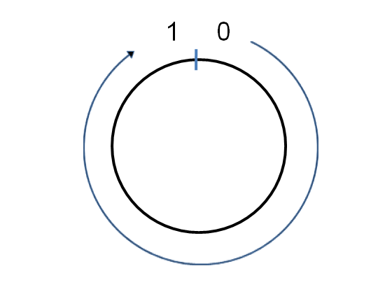
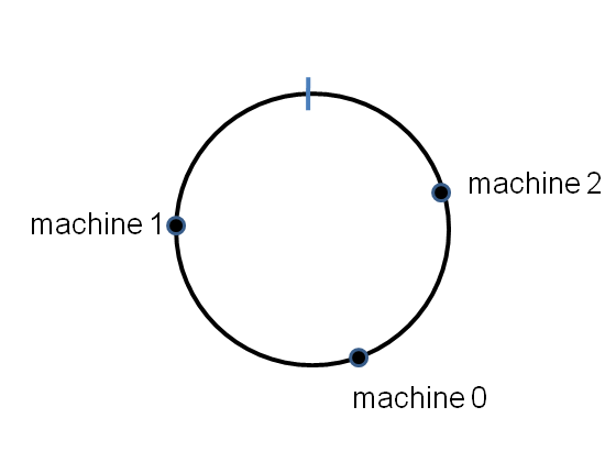
Let’s modify the naive hashing scheme to get a scheme which requires less redistribution of data. Imagine we have a dictionary distributed across two machines using naive hashing, i.e., we compute [tex]\mbox{hash}(k) \mod 2[/tex], and distribute it to machine [tex]0[/tex] if the result is [tex]0[/tex], and to machine [tex]1[/tex] if the result is [tex]1[/tex]. Now we add a third machine to the cluster. We’ll redistribute data by computing [tex]\mbox{hash}(k) \mod 3[/tex], and moving any data for which this value is [tex]0[/tex] to the new machine. It should be easy to convince yourself (and is true, as we’ll prove later!) that one third of the data on both machines [tex]0[/tex] and [tex]1[/tex] will get moved to machine [tex]3[/tex]. So we end up with the data distributed evenly across the three machines and the redistribution step moves far less data around than in the naive approach.

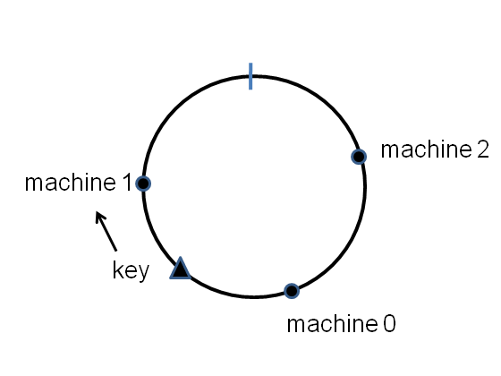
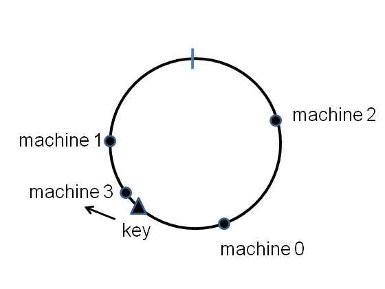
The success of this approach suggests a general scheme for distributing keys across an [tex]n[/tex]-machine cluster. The scheme is to allocate the key [tex]k[/tex] to machine [tex]j[/tex], where [tex]j[/tex] is the largest value in the range [tex]0,\ldots,n-1[/tex] for which [tex]\mbox{hash}(k) \mod (j+1) = 0[/tex]. This scheme is certainly easy to implement. Unfortunately, while it works just fine for clusters of size [tex]n = 2[/tex] and [tex]n = 3[/tex], as we’ve seen, it breaks down when we add a fourth machine. To see why, let’s imagine that we’re expanding from three to four machines. So we imagine the keys are distributed across three machines, and then compute [tex]\mbox{hash}(k) \mod 4[/tex]. If the result is [tex]0[/tex], we move that key to machine [tex]3[/tex]. The problem is that any key for which [tex]\mbox{hash}(k) \mod 2 = 0[/tex] must also have [tex]\mbox{hash}(k) \mod 4 = 0[/tex]. That means that every single key on machine [tex]1[/tex] will necessarily get moved to machine [tex]3[/tex]! So we end up with an uneven distribution of keys across the cluster, not to mention needing to move a large fraction of our data around when doing the redistribution.

With a little thought it should be clear that the underlying problem here is that [tex]4[/tex] and [tex]2[/tex] have a common factor. This suggests a somewhat impractical way of resolving the problem: imagine you only allow clusters whose size is a prime number. That is, you allow clusters of size [tex]2, 3, 5, 7, 11[/tex], and so on, but not any of the sizes inbetween. You could then apply a similar scheme to that described above, but restricted to values of [tex]n[/tex] which are prime. More explicitly, suppose [tex]p_1 < p_2 < p_3 < \ldots < p_n[/tex] is an ascending sequence of primes. Let [tex]p_j[/tex] be the largest prime in this series for which [tex]\mbox{hash}(k) \mod p_j \geq p_{j-1}[/tex]. Then key [tex]k[/tex] is stored on machine [tex]\mbox{hash}(k) \mod p_j[/tex]. Note that we use the convention [tex]p_0 = 0[/tex] to decide which keys to store on machines [tex]0,\ldots,p_1-1[/tex]. Another way of understanding how this modified scheme works is to imagine that we have a cluster of size [tex]p[/tex] (a prime), and then add some more machines to expand the cluster to size [tex]q[/tex] (another prime). We redistribute the keys by computing [tex]\mbox{hash}(k) \mod q[/tex]. If this is in the range [tex]p,\ldots,q-1[/tex], then we move the key to machine number [tex]\mbox{hash}(k) \mod q[/tex]. Otherwise, the key stays where it is. It should be plausible (and we'll argue this in more detail below) that this results in the keys being redistributed evenly across the machines that have been added to the cluster. Furthermore, each of the machines that starts in the cluster contributes equally to the redistribution. The main difference from our earlier approach is that instead of looking for [tex]\mbox{hash}(k) \mod q = 0[/tex], we consider a range of values other than [tex]0[/tex], from [tex]p,\ldots,q-1[/tex]. But that difference is only a superficial matter of labelling, the underlying principle is the same. The reason this scheme works is because the values of [tex]\mbox{hash}(k) \mod p_j[/tex] behave as independent random variables for different primes [tex]p_j[/tex]. To state that a little more formally, we have: Theorem: Suppose [tex]X[/tex] is an integer-valued random variable uniformly distributed on the range [tex]0,\ldots,N[/tex]. Suppose [tex]p_1,\ldots,p_m[/tex] are distinct primes, all much smaller than [tex]N[/tex], and define [tex]X_j \equiv X \mod p_j[/tex]. Then in the limit as [tex]N[/tex] approaches [tex]\infty[/tex], the [tex]X_j[/tex] become independent random variables, with [tex]X_j[/tex] uniformly distributed on the range [tex]0,\ldots,p_j-1[/tex].

The proof of this theorem is an immediate consequence of the Chinese remainder theorem, and I’ll omit it. The theorem guarantees that when we extend the cluster to size [tex]q[/tex], a fraction [tex]1/q[/tex] of the keys on each of the existing machines is moved to each machine being added to the cluster. This results is both an even distribution of machines across the cluster, and the minimal possible redistribution of keys, which is exactly what we desired.

Obviously this hashing scheme for prime-sized clusters is too restrictive to be practical. Although primes occur quite often (roughly one in every [tex]\ln(n)[/tex] numbers near [tex]n[/tex] is prime), it’s still quite a restriction. And it’s going to make life more complicated on large clusters, where we’d like to make the scheme tolerant to machines dropping off the cluster.

Fortunately, there’s an extension of prime-sized hashing which does provide a consistent hashing scheme with all the properties we desire. Here it is. We choose primes [tex]p_0,p_1, \ldots[/tex], all greater than some large number [tex]M[/tex], say [tex]M = 10^9[/tex]. What matters about [tex]M[/tex] is that it be much larger than the largest number of computers we might ever want in the cluster. For each [tex]j[/tex] choose an integer [tex]t_j[/tex] so that:

[tex] \frac{t_j}{p_j} \approx \frac{1}{j+1}. [/tex]

Note that it is convenient to set [tex]t_0 = p_0[/tex]. Our consistent hashing procedure for [tex]n[/tex] machines is to send key [tex]k[/tex] to machine [tex]j[/tex], where [tex]j[/tex] is the largest value such that (a) [tex]j < n[/tex], and (b) [tex]\mbox{hash}(k) \mod p_j[/tex] is in the range [tex]0[/tex] through [tex]t_j-1[/tex]. Put another way, if we add another machine to an [tex]n[/tex]-machine cluster, then for each key [tex]k[/tex] we compute [tex]\mbox{hash}(k) \mod p_n[/tex], and redistribute any keys for which this value is in the range [tex]0[/tex] through [tex]t_n-1[/tex]. By the theorem above this is a fraction roughly [tex]1/(n+1)[/tex] of the keys. As a result, the keys are distributed evenly across the cluster, and the redistributed keys are drawn evenly from each machine in the existing cluster. Performance-wise, for large clusters this scheme is slower than the consistent hashing scheme described in my last post. The slowdown comes because the current scheme requires the computation of [tex]\mbox{hash}(k) \mod p_j[/tex] for [tex]n[/tex] different primes. By contrast, the earlier consistent hashing scheme used only a search of a sorted list of (typically) at most [tex]n^2[/tex] elements, which can be done in logarithmic time. On the other hand, modular arithmetic can be done very quickly, so I don't expect this to be a serious bottleneck, except for very large clusters. Analytically, the scheme in the current post seems to me to likely be preferable - results like the Chinese remainder theorem give us a lot of control over the solution of congruences, and this makes it very easy to understand the behaviour of this scheme and many natural variants. For instance, if some machines are bigger than others, it's easy to balance the load in proportion to machine capacity by changing the threshold numbers [tex]t_j[/tex]. This type of balancing can also be achieved using our earlier approach to consistent hashing, by changing the number of replica points, but the effect on things like the evenness of the distribution and redistribution of keys requires more work to analyse in that case. I'll finish this post as I finished the earlier post, by noting that there are many natural followup questions: what's the best way to cope with servers of different sizes; how to add and remove more than one machine at a time; how to cope with replication and fault-tolerance; how to migrate data when jobs are going on (including backups); and how best to backup a distributed dictionary, anyway? Hopefully it's easy to at least get started on answering these questions at this point. About this post: This is one in a series of posts about the Google Technology Stack – PageRank, MapReduce, and so on. The posts are summarized here, and there is FriendFeed room for the series here. You can subscribe to my blog to follow future posts in the series. If you’re in Waterloo, and would like to attend fortnightly meetups of a group that discusses the posts and other topics related to distributed computing and data mining, drop me an email at mn@michaelnielsen.org.

Today I get back into my post series about the Google Technology Stack, with a more detailed look at distributed dictionaries, AKA distributed key-value stores, AKA distributed hash tables. What we’d like to do is store a dictionary of key-value pairs [tex](k_1,v_1),(k_2,v_2),\ldots[/tex] across a cluster of computers, preferably in a way that makes it easy to manipulate the dictionary without having to think about the details of the cluster.

The reason we’re interested in distributed dictionaries is because they’re used as input and output to the MapReduce framework for distributed computing. Of course, that’s not the only reason distributed dictionaries are interesting – they’re useful for many other purposes (e.g., distributed caching). But for the purposes of this post, we’ll imagine our distributed dictionaries are being used as the input and output from a MapReduce job.

I’ll describe two ways of implementing distributed dictionaries. The first is a naive method that’s simple and works pretty well. Then I’ll introduce an improved method called “consistent hashing”. Consistent hashing isn’t the final word in distributed dictionaries, but it’s a good start. All the usual caveats apply to the post: I’m still learning this stuff, and corrections, improvements, etcetera are welcome!

Let’s start with the naive method. Suppose we have a cluster of [tex]n[/tex] computers. We number the computers [tex]0,1,2,\ldots,n-1[/tex], and then store the key-value pair [tex](k,v)[/tex] on computer number [tex]\mbox{hash}(k) \mod n[/tex], where [tex]\mbox{hash}(\cdot)[/tex] is a hash function. If we’re using a good hash function, then [tex]\mbox{hash}(k) \mod n[/tex] is uniform across [tex]0,\ldots,n-1[/tex] for any reasonable distribution of keys. This ensures our distributed dictionary is spread evenly across the computers in our cluster, and doesn’t build up too much on any individual computer.

As a brief Pythonic aside, Python’s builtin hash function doesn’t have this property of spreading keys out uniformly. It sometimes takes similar key strings to similar hash values. Here’s a typical sample (results may vary on your machine):

hash("answer0") -> 1291065813204512909

hash("answer1") -> 1291065813204512908

hash("answer2") -> 1291065813204512911

What this means is that you can’t depend on Python’s builtin hash function to spread keys and values uniformly across the cluster. In principle, far better hash functions are available through the hashlib library, functions which do offer guarantees about uniformity. Those functions are quite a lot slower than hash – I did a little benchmark comparing hash to the hashlib.md5 hash, and found that hash was about ten times faster. We’ll use the hashlib library, although in practice I imagine you’d want something faster, but without the disadvantages of hash. End of Pythonic aside.

Naive hash-based distributed dictionaries are simple, but they have serious limitations. Imagine you’re using a cluster of computers to crawl the web. You store the results of your crawl in a distributed dictionary. But as the size of the crawl grows, you’ll want to add machines to your cluster. Suppose you add even just a single machine. Instead of computing [tex]\mbox{hash}((k) \mod n[/tex] we’re now computing [tex]\mbox{hash}(k) \mod (n+1)[/tex]. The result is that each key-value pair will get reallocated completely at random across the cluster. You’ll end up moving a fraction [tex]n/(n+1)[/tex] of your data to new machines – i.e., nearly all of it. This will be slow, and might potentially be expensive. It’s also potentially inconvenient if jobs are being carried out. Similar problems arise if you add a larger block of machines to the cluster, or if you lose some machines (e.g., if some of the machines fail). You get the idea.

Consistent hashing solves these problems. Like naive hashing, consistent hashing spreads the distributed dictionary evenly across the cluster. But unlike naive hashing, consistent hashing requires only a relatively small amount of data to be moved: if you add a machine to the cluster, only the data that needs to live on that machine is moved there; all the other data stays where it is.

To understand how consistent hashing works, imagine wrapping the unit interval [tex][0,1)[/tex] onto a circle:

Suppose we number the machines [tex]0,\ldots,n-1[/tex]. If the hash function has range [tex][0,R)[/tex] then we rescale the hash function via [tex]x \rightarrow \mbox{hash}(x)/R[/tex], so that the hash function maps into the range [tex][0,1)[/tex], i.e., effectively onto the circle. Then we can hash machine number [tex]j[/tex] to a point [tex]\mbox{hash}(j)[/tex] on the circle, for each machine in the range [tex]j = 0,1,\ldots,n-1[/tex]. Here’s what it might look like for an [tex]n=3[/tex] machine cluster:

The points will be randomly distributed around the circle. Now suppose we have a key-value pair we want to store in the distributed dictionary. We simply hash the key onto the circle, and then store the key-value pair on the first machine that appears clockwise of the key’s hash point. E.g., for the key shown here, the key-value pair is stored on machine number [tex]1[/tex]:

Because of the uniformity of the hash function, a fraction roughly [tex]1/n[/tex] of the key-value pairs will get stored on any single machine.

Now imagine we add an extra machine into the cluster. It goes to the point [tex]\mbox{hash}(n)[/tex]:

Most of the key-value pairs are completely unaffected by this change. But we can see that some of the key-value pairs that were formerly stored on machine [tex]1[/tex] (including our example key-value pair) will need to be moved to the new machine. But the fraction that needs to be moved will typically be [tex]1/(n+1)[/tex] of the total, a much smaller fraction than was the case for naive hashing.

The procedure I’ve described isn’t quite ideal, for a couple of reasons. First, the distribution of keys can be pretty irregular. If, for example, two of the machines – say [tex]j[/tex] and [tex]j'[/tex] – get mapped to very nearby points on the circle, then one of those machines may end up with very few of the keys, and some other machines with correspondingly more. It’s not that serious a problem, but why waste even a single machine? Second, when a machine is added to the cluster, all the keys redistributed to that machine come from just one other machine. Ideally, the keys would come in a more balanced way from several other machines.

Both these problems are easily resolved. Instead of mapping machine number [tex]j[/tex] to a single point on the circle, we’ll map it to multiple points (“replicas”). In particular, let’s imagine that for each machine we pick out [tex]r[/tex] points, by hashing [tex](j,0), (j,1),\ldots(j,r-1)[/tex] onto the circle. Otherwise, everything works exactly as before. By adding these replicas, we increase both the uniformity with which key-value pairs are mapped to machines, and also ensure that when a machine is added to the cluster, a smaller number of keys ([tex]\Theta(1/rn)[/tex]) are redistributed to that machine, from each of [tex]\Theta(r)[/tex] other machines in the cluster.

Here’s a simple Python program that implements consistent hashing. It’s largely self-explanatory; if you’d like to play around with it, I recommend reading the doc string for the ConsistentHash class.

'''consistent_hashing.py is a simple demonstration of consistent
hashing.'''

import bisect
import hashlib

class ConsistentHash:
  '''ConsistentHash(n,r) creates a consistent hash object for a 
  cluster of size n, using r replicas.

  It has three attributes. num_machines and num_replics are
  self-explanatory.  hash_tuples is a list of tuples (j,k,hash), 
  where j ranges over machine numbers (0...n-1), k ranges over 
  replicas (0...r-1), and hash is the corresponding hash value, 
  in the range [0,1).  The tuples are sorted by increasing hash 
  value.

  The class has a single instance method, get_machine(key), which
  returns the number of the machine to which key should be 
  mapped.'''

  def __init__(self,num_machines=1,num_replicas=1):
    self.num_machines = num_machines
    self.num_replicas = num_replicas
    hash_tuples = [(j,k,my_hash(str(j)+"_"+str(k))) \
                   for j in range(self.num_machines) \
                   for k in range(self.num_replicas)]
    # Sort the hash tuples based on just the hash values
    hash_tuples.sort(lambda x,y: cmp(x[2],y[2]))
    self.hash_tuples = hash_tuples

  def get_machine(self,key):
    '''Returns the number of the machine which key gets sent to.'''
    h = my_hash(key)
    # edge case where we cycle past hash value of 1 and back to 0.
    if h > self.hash_tuples[-1][2]: return self.hash_tuples[0][0]
    hash_values = map(lambda x: x[2],self.hash_tuples)
    index = bisect.bisect_left(hash_values,h)
    return self.hash_tuples[index][0]

def my_hash(key):
  '''my_hash(key) returns a hash in the range [0,1).'''
  return (int(hashlib.md5(key).hexdigest(),16) % 1000000)/1000000.0

def main():
  ch = ConsistentHash(7,3)
  print "Format:"
  print "(machine,replica,hash value):"
  for (j,k,h) in ch.hash_tuples: print "(%s,%s,%s)" % (j,k,h)
  while True:
    print "\nPlease enter a key:"
    key = raw_input()
    print "\nKey %s maps to hash %s, and so to machine %s" \
        % (key,my_hash(key),ch.get_machine(key))

if __name__ == "__main__": main()

Having understood the basics of consistent hashing, there’s many natural followup questions: what’s the best way to cope with servers of different sizes; how to add and remove more than one machine at a time; how to cope with replication and fault-tolerance; how to migrate data when jobs are going on (including backups); and how best to backup a distributed dictionary, anyway? Hopefully it’s easy to get started on answering these questions at this point.

Let me finish up with a little background history. Consistent hashing was introduced pretty recently, in 1997, in a pair of papers, one describing the theory, the other about implementation. Note that the original papers were focused on applications to caching on the world wide web, not to distributed computing applications like MapReduce. A good (and funny!) basic introduction to consistent hashing is here. It’s now widely used inside services like the popular memcached caching system, and Amazon’s Dynamo key-value store.

About this post: This is one in a series of posts about the Google Technology Stack – PageRank, MapReduce, and so on. The posts are summarized here, and there is FriendFeed room for the series here. The posts are based on fortnightly meetups of a small group in Waterloo – email me (mn@michaelnielsen.org) if you’re local and interested in attending. Subscribe to my blog to follow future posts in the series.

How do computers translate texts from one language to another? Human translators use a great deal of detailed knowledge about how the world works to correctly translate all the different meanings the same word or phrase can have in different contexts. This makes automated translation seem like it might be a hard problem to solve, the kind of problem that may require genuine artificial intelligence. Yet although translators like Google Translate and Yahoo!’s Babel Fish are far from perfect, they do a surprisingly good job. How is that possible?

In this post, I describe the basic ideas behind the most successful approach to automated machine translation, an approach known as statistical machine translation. Statistical machine translation starts with a very large data set of good translations, that is, a corpus of texts (e.g., United Nations documents) which have already been translated into multiple languages, and then uses those texts to automatically infer a statistical model of translation. That statistical model is then applied to new texts to make a guess as to a reasonable translation.

I’m not an expert in statistical machine translation. I’ve written these notes to help me internalize the basic ideas of the area. However, I hope the notes are useful to others as an introductory overview of statistical machine translation, and as a starting place to learn more.

Formulating the problem

Imagine you’re given a French text, [tex]f[/tex], and you’d like to find a good English translation, [tex]e[/tex]. There are many possible translations of [tex]f[/tex] into English, of course, and different translators will have different opinions about what the best translation, [tex]e[/tex], is. We can model these differences of opinion with a probability distribution [tex]\mbox{pr}(e|f)[/tex] over possible translations, [tex]e[/tex], given that the French text was [tex]f[/tex]. A reasonable way of choosing the “best” translation is to choose [tex]e[/tex] which maximizes the conditional probability [tex]\mbox{pr}(e|f)[/tex].

The problem with this strategy is that we don’t know the conditional probability [tex]\mbox{pr}(e|f)[/tex]. To solve this problem, suppose we’re in possession of an initial corpus of documents that are in both French and English, e.g., United Nations documents, or the Canadian parliamentary proceedings. We’ll use that corpus to infer a model estimating the conditional probabilities [tex]\mbox{pr}(e|f)[/tex]. The model we’ll construct is far from perfect, but with a large and high quality initial corpus, yields pretty good translations. To simplify the discussion we assume [tex]e[/tex] and [tex]f[/tex] are single sentences, and we’ll ignore punctuation; obviously, the translator can be applied serially to a text containing many sentences.

Now, how do we start from the corpus and infer a model for [tex]\mbox{pr}(e|f)[/tex]? The standard approach is to use Bayes’ theorem to first rewrite [tex]\mbox{pr}(e|f)[/tex] as

[tex] \mbox{pr}(e|f) = \frac{\mbox{pr}(f|e) \mbox{pr}(e)}{\mbox{pr}(f)}. [/tex]

Because [tex]f[/tex] is fixed, the maximization over [tex]e[/tex] is thus equivalent to maximizing

[tex] \mbox{pr}(f|e) \mbox{pr}(e). [/tex]

What we’re going to do is to use our data set to infer models of [tex]\mbox{pr}(f|e)[/tex] and [tex]\mbox{pr}(e)[/tex], and then use those models to search for [tex]e[/tex] maximizing [tex]\mbox{pr}(f|e) \mbox{pr}(e)[/tex].

The procedure outlined in the last paragraph seems a priori like a strange thing to do. Why not save time and difficulty by inferring a model of [tex]\mbox{pr}(e|f)[/tex] and then maximizing directly? It turns out that the procedure I described actually works quite a bit better. Now, to be blunt, I don’t entirely understand the explanations of this I’ve read in the published literature. But what I think is going on is as follows. It turns out that if we work directly with [tex]\mbox{pr}(e|f)[/tex], then many malformed English sentences [tex]e[/tex] are given a high probability by our model. You’ll see why this is the case later – it’s obvious from the construction – but for now just accept that’s the case. If we worked directly with [tex]\mbox{pr}(e|f)[/tex] those sentences would often be issued as “translations”, which is no good. Now, why should maximizing [tex]\mbox{pr}(f|e) \mbox{pr}(e)[/tex] work any better? After all, both [tex]\mbox{pr}(f|e)[/tex] and [tex]\mbox{pr}(e)[/tex] may give high probabilistic weight to sentences [tex]e[/tex] which are not well-formed. So what gives? I think there are two things going on. First, although [tex]\mbox{pr}(f|e)[/tex] and [tex]\mbox{pr}(e)[/tex] may give high weight to malformed sentences [tex]e[/tex], the models are constructed very differently. For both to give high weight simultaneously, it’s quite unlikely that [tex]e[/tex] is malformed. Second, we can build grammatical checks directly into the construction of [tex]\mbox{pr}(e)[/tex], so very few malformed sentences have high values for [tex]\mbox{pr}(e)[/tex]. We won’t actually do that in this post, but it’s relatively straightforward to do.

We’ve broken machine translation up into three problems: (1) build a language model which allows us to estimate [tex]\mbox{pr}(e)[/tex]; (2) build a translation model which allows us to estimate [tex]\mbox{pr}(f|e)[/tex]; and (3) search for [tex]e[/tex] maximizing the product [tex]\mbox{pr}(f|e)\mbox{pr}(e)[/tex]. Each of these problems is itself a rich problem which can be solved in many different ways. In the next three sections I’ll describe simple approaches to solving each of the three problems.

The language model

Suppose we break an English sentence [tex]e[/tex] up into words [tex]e = e_1e_2\ldots e_m[/tex]. Then we can write the probability for [tex]e[/tex] as a product of conditional probabilities:

[tex] \mbox{pr}(e) = \prod_{j=1}^m \mbox{pr}(e_j|e_1,\ldots,e_{j-1}) [/tex]

So, for example, in the sentence fragment “To be or not to…”, you would probably assign a very high conditional probability to the final word being “be”, certainly much higher than the probability of its occurrence at a random point in a piece of text.

The challenge in building a good language model [tex]\mbox{pr}(e)[/tex] is that there are so many distinct conditional probabilities that need to be estimated. To simplify the problem we’ll make some assumptions about the form of the probabilities. The most drastic assumption we could make is to assume that the probability of seeing a word is independent of what came before it, i.e.,

[tex] \mbox{pr}(e_j|e_1,\ldots,e_{j-1}) = \mbox{pr}(e_j), [/tex]

so

[tex] \mbox{pr}(e) = \prod_{j=1}^m \mbox{pr}(e_j). [/tex]

We could estimate the probabilities [tex]\mbox{pr}(e_j)[/tex] by taking a very large corpus of English text, and counting words. The problem is that this model is not very realistic. A more realistic model is the bigram model, which assumes that the probability of a word occurring depends only on the word immediately before it:

[tex] \mbox{pr}(e_j|e_1,\ldots,e_{j-1}) = \mbox{pr}(e_j|e_{j-1}). [/tex]

More realistic still is the trigram model, which assumes that the probability of a word occurring depends only on the two words immediately before it:

[tex] \mbox{pr}(e_j|e_1,\ldots,e_{j-1}) = \mbox{pr}(e_j|e_{j-2},e_{j-1}). [/tex]

To make the discussion which follows as concrete as possible, let’s concentrate on the problem of how to estimate conditional probabilities in the bigram model. Similar remarks can be made for the trigram model. The obvious way to proceed is to take a large corpus of English text, count the number of occurrences [tex]\#(e_1,e_2)[/tex] of a particular word pair in that corpus, and then set [tex]\mbox{pr}(e_2|e_1) = \#(e_1,e_2)/\#(e_1)[/tex].

The problem with this procedure is that there are a lot of bigrams. If we assume that there are 50,000 words in English, say, then there are 2.5 billion possible bigrams. Even if you take a large corpus of training data (say, a billion words), it’s reasonably likely that there will be some bigrams which don’t appear in your corpus, and thus are assigned zero probability, yet which you would a priori like to appear in translations of some French sentences. That is, this kind of training procedure is likely to underestimate the probability of bigrams which don’t appear in the training set, and overestimate the probability of those which do. The problem is even worse for trigrams.

There’s no obvious best solution to this problem. Many different ad hoc solutions have been tried, and my quick survey of the literature suggests that there’s as yet no broad agreement about the best way of solving the problem. To give you the flavour of the solutions people use, though, let me describe two basic approaches, adapted from the survey in section 2.3 of Philip Clarkson’s PhD thesis.

The first approach is to move away from a pure bigram model, and instead to use linear interpolation between the monogram and bigram models. A large and diverse enough corpus of text is likely to give pretty good estimates for nearly all single-word probabilities [tex]\mbox{pr}(e_1)[/tex]. So one way of estimating [tex]\mbox{pr}(e_2|e_1)[/tex] is as:

[tex] \mbox{pr}(e_2|e_1) = \lambda \frac{\#(e_2)}{N} + (1-\lambda) \frac{\#(e_1,e_2)}{\#(e_1)}, [/tex]

where [tex]N[/tex] is the total number of words in the corpus. [tex]\lambda[/tex] is a parameter in the range [tex]0 < \lambda < 1[/tex] which needs to be determined. This can be done using a second corpus of text, and setting [tex]\lambda[/tex] so that the average probability of the bigrams in that corpus is maximized. A second approach is to apply a discount factor to the conditional probabilities for the bigrams which appear in the training corpus, essentially reducing their probability. The easist way to proceed is simply to multiply them all by some constant [tex]c[/tex] in the range [tex]0 < c < 1[/tex], and then to spread the remaining probability [tex]1-c[/tex] uniformly over all bigrams [tex](e_1,e_2)[/tex] which don't appear in the corpus.

Exercises

• The constant [tex]c[/tex] can be viewed as an estimate of the fraction of all English bigrams that appear in the training corpus. How might you go about obtaining an estimate for [tex]c[/tex]?

To conclude this section, let me mention that the problem of building a good language model is also of great interest to people working on speech recognition software. In fact, much of the research literature on language models can be applied equally to either speech recognition or statistical machine translation.

The translation model

Note: English is my only language, which makes it hard for me to construct translation examples! All my examples are taken from a paper by Brown et al.

In this section we’ll construct a simple translation model allowing us to compute [tex]\mbox{pr}(f|e)[/tex]. Intuitively, when we translate a sentence, words in the source text generate (possibly in a context-dependent way) words in the target language. In the sentence pair (Jean aime Marie | John loves Mary) we intuitively feel that John corresponds to Jean, loves to aime, and Mary to Marie. Of coure, there is no need for the word correspondence to be one-to-one, nor for the ordering of words to be preserved. Sometimes, a word in English may generate two or more words in French; sometimes it may generate no word at all.

Despite these complications, the notion of a correspondence between words in the source language and in the target language is so useful that we’ll formalize it through what is called an alignment. Rather than give a precise definition, let me explain alignments through an example, the sentence pair (Le chien est battu par Jean | John (6) does beat (3,4) the (1) dog (2)). In this example alignment, the numbers in parentheses tell us that John corresponds to the 6th word in the French sentence, i.e., Jean. The word does has no trailing parentheses, and so doesn’t correspond to any of the words in the French sentence. However, beat corresponds to not one, but two separate words in the French sentence, the 3rd and 4th words, est and battu. And so on.

Two notions derived from alignments are particularly useful in building up our translation model. The first is fertility, defined as the number of French words generated by a given English word. So, in the example above, does has fertility [tex]0[/tex], since it doesn’t generate anything in the French sentence. On the other hand, beat has fertility [tex]2[/tex], since it generates two separate words in the French sentence.

The second notion is distortion. In many sentences, the English word and its corresponding French word or words appear in the same part of the sentence – near the beginning, perhaps, or near the end. We say that such words are translated roughly undistorted, while words which move a great deal have high distortion. We’ll encoude this notion more formally shortly.

We’ll build up our translation model using some simple parameters related to fertility and distortion:

• The fertility probability [tex]\mbox{pr}(n|e)[/tex], the probability that the English word [tex]e[/tex] has fertility [tex]n[/tex].
• The distortion probability [tex]\mbox{pr}(t|s,l)[/tex], which is the probability that an English word at position [tex]s[/tex] corresponds to a French word at position [tex]t[/tex] in a French sentence of length [tex]l[/tex].
• The translation probability [tex]\mbox{pr}(f|e)[/tex], one for each French word [tex]f[/tex] and English word [tex]e[/tex]. This should not be confused with the case when [tex]f[/tex] and [tex]e[/tex] are sentences!

I’ve described the translation model as a way of computing [tex]\mbox{pr}(f|e)[/tex], where [tex]e[/tex] is an English sentence, and [tex]f[/tex] is a French sentence. In fact, we’re going to modify that definition a little, defining the translation model as the probability [tex]\mbox{pr}(f,a|e)[/tex] that the French sentence [tex]f[/tex] is the correct translation of [tex]e[/tex], with a particular alignment, which we’ll denote by [tex]a[/tex]. I’ll return to the question of how this change in definition affects translation in the next section. Rather than specify the probability for our translation model formally, I’ll simply show how it works for the example alignment (Le chien est battu par Jean |John (6) does beat (3,4) the (1) dog (2)):

[tex]\mbox{pr}(1|John) \times \mbox{pr}(Jean|John) \times \mbox{pr}(6|1,6) \times [/tex]

[tex]\mbox{pr}(0|does) \times [/tex]

[tex]\mbox{pr}(2|beat) \times \mbox{pr}(est|beat) \times \mbox{pr}(3|3,6) \times \mbox{pr}(battu|beat) \times \mbox{pr}(4|3,6) \times [/tex]

[tex]\mbox{pr}(1|the) \times \mbox{pr}(Le|the) \times \mbox{pr}(1|5,6) \times [/tex]

[tex]\mbox{pr}(1|dog) \times \mbox{pr}(chien|dog) \times \mbox{pr}(2|6,6) \times [/tex]

[tex]\mbox{pr}(1|) \times \mbox{pr}(par|) [/tex]

This should be self-explanatory except the final line, for the French word par. This word has no corresponding word in the English sentence, which we model using a special word [tex][/tex].

What remains to be done is to estimate the parameters used in constructing the translation model – the fertility, distortion and translation probabilities. I’ll briefly outline an iterative procedure that can be used to do this estimation. It starts with a simple guess of the parameters. E.g., we might guess that the distortion probabilities [tex]\mbox{pr}(t|s,l) = 1/l[/tex] are uniform across the sentence. Similar guesses could be made for the other parameters. For each pair [tex](e,f)[/tex] of sentences in our corpus we can use this guess to compute the probability for all possible alignments between the sentences. We then estimate the “true” alignment to be whichever alignment has highest probability. Applying this procedure to the entire corpus gives us many estimated alignments. We can then use those estimated alignments to compute new estimates for all the parameters in our model. E.g., if we find that [tex]1/10[/tex]th of the alignments of sentences of length [tex]25[/tex] have the first word mapped to the first word then our new estimate for [tex]\mbox{pr}(1|1,25) = 1/10[/tex]. This gives us a procedure for iteratively updating the parameters of our model, which can be repeated many times. Empirically we find (and it can be proved) that the parameters gradually converge to a fixed point.

Exercises

• A problem I’ve glossed over above is figuring out which sentences in the English corpus correspond to which sentences in the French corpus. How could you figure out which sentences correspond to which? What would be the effect of mistakes?

Searching for the maximizing [tex]e[/tex]

In my introductory remarks I explained how translation from French to English can be viewed as the problem of finding [tex]e[/tex] which maximizes [tex]\mbox{pr}(e|f)[/tex], and that this was equivalent to maximizing [tex]\mbox{pr}(f|e)\mbox{pr}(e)[/tex]. Let’s revisit the reasoning which led to that framing of the problem, and recast it in a form more amenable to our translation model based on alignments. Instead of searching for [tex]e[/tex] which maximizes [tex]\mbox{pr}(e|f)[/tex], let’s instead search for a pair [tex](e,a)[/tex] which maximizes [tex]\mbox{pr}(e,a|f)[/tex]. Using Bayes’ theorem this is equivalent to finding [tex](e,a)[/tex] which maximizes

[tex] \mbox{pr}(e,a|f) = \frac{\mbox{pr}(f,a|e) \mbox{pr}(e)} {\mbox{pr}(f)}. [/tex]

As earlier, we can omit the factor [tex]\mbox{pr}(f)[/tex] in the denominator, and so our search is equivalent to finding a pair [tex](e,a)[/tex] which maximizes

[tex] \mbox{pr}(f,a|e) \mbox{pr}(e) [/tex]

Our translation problem is to find [tex](e,a)[/tex] maximizing this expression. Unfortunately, there are far too many possibility to do an exhaustive search. But there are some heauristics which work pretty well. One is to use a greedy algorithm which gradually builds up partial translations and alignments. Consider the following partial translations and alighments:

(Jean aime Marie | John (1) *)

(Jean aime Marie | * loves (2) *)

(Jean aime Marie | Petroleum (1) *)

Using the translation and language models described earlier we can compute the probabilities for each of these partial alignments, and so compute the product [tex]\mbox{pr}(f,a|e) \mbox{pr}(e)[/tex]. It would be very surprising if the first two candidates weren’t assigned a high probability, and the third example a very low probability. Our heuristic for search is thus to maintain a stack of promising partial translations and alignments, and to continually extend those partial translations and alignments until we find a complete translation and alignment with a significantly higher probability than any of the partial alignments.

Commentary

Rather than argue about whether this algorithm is better than that algorithm, all you have to do is get ten times more training data. And now all of a sudden, the worst algorithm … is performing better than the best algorithm on less training data. Worry about the data first before you worry about the algorithm.

— Peter Norvig, Director of Research at Google, as reported by Greg Linden.

That completes our description of a simple statistical machine translation system. The system I’ve described is essentially the same as the system described in 1990 by Brown et al at IBM research, a system which translated roughly half of all sentences in an acceptable way! Personally, I find it remarkable that such simple ideas can be used to make so much progress on what appears to be an enormously difficult problem. (I’ll describe other examples in future posts.) Furthermore, although the basic ideas remain the same, many improvements to these ideas have been made since 1990. The biggest single advance seems to have been a movement away from words as the unit of language, and towards phrase-based models, which give greatly improved performance.

If you’re interested in understanding more, I strongly suggest checking out an accessible and very influential 1993 follow-up paper from the IBM group, which describes a whole plethora of translation models. I don’t have a single canonical reference to give on phrase-based statistical translation models, but found several of the top hits at Google Scholar quite informative. Finally, and just for fun, I recommend Peter Norvig’s excellent short introduction to automatic spelling correction, which uses similar ideas in a much (!) simpler setting, but has the big advantage that it is illustrated by real code.

About this post: This is one in a series of posts about the Google Technology Stack – PageRank, MapReduce, and so on. The posts are summarized here, and there is FriendFeed room for the series here. Subscribe to my blog to follow future posts in the series.

In this post I explain how to compute PageRank using the MapReduce approach to parallelization. This gives us a way of computing PageRank that can in principle be automatically parallelized, and so potentially scaled up to very large link graphs, i.e., to very large collections of webpages. In this post I describe a single-machine implementation which easily handles a million or so pages. In future posts we’ll use a cluster to scale out much further – it’ll be interesting to see how far we can get.

I’ve discussed PageRank and MapReduce at length in earlier posts – see here for MapReduce, and here and here for PageRank – so in this post we’ll just quickly review the basic facts. Let’s start with PageRank. The idea is that we number webpages [tex]0,\ldots,n-1[/tex]. For webpage number [tex]j[/tex] there is an associated PageRank [tex]q_j[/tex] which measures the importance of page [tex]j[/tex]. The vector [tex]q = (q_0,\ldots,q_{n-1})[/tex] of PageRanks is a probability distribution, i.e., the PageRanks are numbers between [tex]0[/tex] and [tex]1[/tex], and sum up to one, in total. The PageRank [tex]q_j[/tex] measures the importance of page [tex]j[/tex]; the bigger the PageRank, the more important the page.

How is the PageRank vector [tex]q[/tex] computed? I’ll just describe the mathematical upshot here; the full motivation in terms of a crazy websurfer who randomly surfs the web is described in an earlier post. The upshot is that the PageRank vector [tex]q[/tex] can be defined by the equation (explanation below):

[tex] q \leftarrow M^j P. [/tex]

What this equation represents is a starting distribution [tex]P[/tex] for the crazy websurfer, and then [tex]j[/tex] steps of “surfing”, with each action of [tex]M[/tex] representing how the distribution changes in a single step. [tex]P[/tex] is an [tex]n[/tex]-dimensional vector, and [tex]M[/tex] is an [tex]n \times n[/tex] matrix whose entries reflect the link structure of the web in a way I’ll make precide below. The PageRank [tex]q[/tex] is defined in the limit of large [tex]j[/tex] – in our examples, convergence typically occurs for [tex]j[/tex] in the range [tex]10[/tex] to [tex]30[/tex]. You might wonder how [tex]P[/tex] is chosen, but part of the magic of PageRank is that it doesn’t matter how [tex]P[/tex] is chosen, provided it’s a probability distribution. The intuition is that the starting distribution for the websurfer doesn’t matter to the websurfer’s long-run behaviour. We’ll start with the uniform probability distribution, [tex]P = (1/n,1/n,\ldots)[/tex], since it’s easy to generate.

How is the matrix [tex]M[/tex] defined? It can be broken up into three pieces

[tex] M = s A + s D + t E, [/tex]

including: a contribution [tex]sA[/tex] representing the crazy websurfer randomly picking links to follow; a contribution [tex]sD[/tex] due to the fact that the websurfer can’t randomly pick a link when they hit a dangling page (i.e., one with no outbound links), and so something else needs to be done in that case; and finally a contribution [tex]tE[/tex] representing the websurfer getting bored and “teleporting” to a random webpage.

We’ll set [tex]s = 0.85[/tex] and [tex]t = 1-s = 0.15[/tex] as the respective probabilities for randomly selecting a link and teleporting. See this post for a discussion of the reasons for this choice.

The matrix [tex]A[/tex] describes the crazy websurfer’s linkfollowing behaviour, and so, in some sense, encodes the link structure of the web. In particular, suppose we define [tex]\#(j)[/tex] to be the number of links outbound from page [tex]j[/tex]. Then [tex]A_{kj}[/tex] is defined to be [tex]0[/tex] if page [tex]j[/tex] does not link to page [tex]k[/tex], and [tex]1/\#(j)[/tex] if page [tex]j[/tex] does link to page [tex]k[/tex]. Stated another way, the entries of the [tex]j[/tex]th column of [tex]A[/tex] are zero, except at locations corresponding to outgoing links, where they are [tex]1/\#(j)[/tex]. The intuition is that [tex]A[/tex] describes the action of a websurfer at page [tex]j[/tex] randomly choosing an outgoing link.

The matrix [tex]D[/tex] is included to deal with dangling pages, i.e., pages with no outgoing links. For such pages it is obviously ambiguous what it means to choose an outgoing link at random. The conventional resolution is to choose another page uniformly at random from the entire set of pages. What this means is that if [tex]j[/tex] is a dangling page, then the [tex]j[/tex]th column of [tex]D[/tex] should have all its entries [tex]1/n[/tex], otherwise, if [tex]j[/tex] is not dangling, all the entries should be zero. A compact way of writing this is

[tex] D = e d^T/ n, [/tex]

where [tex]d[/tex] is the vector of dangling pages, i.e., the [tex]j[/tex]th entry of [tex]d[/tex] is [tex]1[/tex] if page [tex]j[/tex] is dangling, and otherwise is zero. [tex]e[/tex] is the vector whose entries are all [tex]1[/tex]s.

The final piece of [tex]M[/tex] is the matrix [tex]E[/tex], describing the bored websurfer teleporting somewhere else at random. This matrix has entries [tex]1/n[/tex] everywhere, representing a uniform probability of going to another webpage.

Okay, that’s PageRank in a mathematical nutshell. What about MapReduce? Again, I’ll just remind you of the basic details – if you want an introduction, see this post. MapReduce is one of those ideas where understanding is really helped by first working through an example, rather than starting with an abstract description, like I’m about to give, so if you’re not familiar with MapReduce, I strongly suggest reading the earlier post.

The input to a MapReduce job is a set of (input_key,input_value) pairs. Each pair is used as input to a function mapper(input_key,input_value) which produces as output a list of intermediate keys and intermediate values:

[(intermediate_key,intermediate_value),
 (intermediate_key',intermediate_value'),
 ...]

The output from all the different input pairs is then sorted, so that intermediate values associated with the same intermediate_key are grouped together in a list of intermediate values. The reducer(intermediate_key,intermediate_value_list) function is then applied to each intermediate key and list of intermediate values, to produce the output from the MapReduce job.

Computing PageRank with MapReduce

Okay, so how can we compute PageRank using MapReduce? The approach we’ll take is to use MapReduce to repeatedly multiply a vector by the matrix [tex]M[/tex]. In particular, we’re going to show that if [tex]p[/tex] is a probability distribution, then we can easily compute [tex]Mp[/tex] using MapReduce. We can thus compute [tex]M^jP[/tex] using repeated invocations of MapReduce. Those invocations have to be done serially, but the individual MapReduce jobs are themselves all easily parallelized, and so we can potentially get a speedup by running those jobs on a big cluster. Much more about doing that in later posts.

The nub of the problem, then, is figuring out how to compute [tex]Mp[/tex], given a starting probability distribution [tex]p[/tex]. Let’s start out with a rough approach that gets the basic idea right, essentially using MapReduce to compute [tex]Ap[/tex]. We’ll see below that it’s easy to fix this up to take dangling nodes and teleportation into account. The fix involves introducing an additional MapReduce job, though, so each multiplication step [tex]p \rightarrow Mp[/tex] actually involves two MapReduce jobs, not just one. For now, though, let’s concentrate on roughing out a MapReduce job that computes [tex]Ap[/tex].

As input to the MapReduce computation, we’ll use (key,value) pairs where the key is just the number of the webpage, let’s call it j, and value contains several items of data describing the page, including [tex]p_j[/tex], the number [tex]\#(j)[/tex] of outbound webpages, and a list [k_1,k_2,...] of pages that j links to.

For each of the pages k_l that j links to, the mapper outputs an intermediate key-value pair, with the intermediate key being k_l and the value just the contribution [tex]p_j/\#(j)[/tex] made to the PageRank. Intuitively, this corresponds to the crazy websurfer randomly moving to page k_l, with the probability [tex]p_j/\#(j)[/tex] combining both the probability [tex]p_j[/tex] that they start at page [tex]j[/tex], and the probability [tex]p_j/\#(j)[/tex] that they move to page k_l.

Between the map and reduce phases, MapReduce collects up all intermediate values corresponding to any given intermediate key, k, i.e., the list of all the probabilities of moving to page k. The reducer simply sums up all those probabilities, outputting the result as the second entry in the pair (k,p_k'), and giving us the entries of [tex]Ap[/tex], as was desired.

To modify this so it computes [tex]Mp[/tex] we need to make three changes.

The first change is to make sure we deal properly with dangling pages, i.e., we include the term [tex]sD[/tex]. One possible way is to treat dangling pages as though they have outgoing links to every single other page, [0,1,2,...]. While this works, it would require us to maintain many very large lists of links, and would be extremely inefficient.

A better way to go is to use our earlier expression [tex]D = e d^T/n[/tex], and thus [tex]Dp = e (d\cdot p)/n[/tex], where [tex]d \cdot p[/tex] is the inner product between the vector [tex]d[/tex] of dangling pages, and [tex]p[/tex]. Computing [tex]Dp[/tex] then really boils down to computing [tex]d \cdot p[/tex].

We can compute [tex]d \cdot p[/tex] using a separate MapReduce job which we run first. This job computes the inner product, and then passes it as a parameter to the second MapReduce job, which is based on the earlier rough description, and which finishes off the computation. This first MapReduce job uses the same input as the earlier job – a set of keys j corresponding to pages, and values describing the pages, i.e., containing the value for p_j, and a description of the outbound links from page j. If page j is dangling the mapper outputs the intermediate pair (1,p_j), otherwise it outputs nothing. All the intermediate keys are the same, so the reducer acts on just one big list, summing up all the values p_j for dangling pages, giving us the inner product we wanted.

As an aside, while this prescription for computing the inner product using MapReduce is obviously correct, you might worry about the fact that all the intermediate keys have the same value. This means all the intermediate values will go to a single reducer, running on just one machine in the cluster. If there are a lot of dangling pages, that means a lot of communication and computation overhead associated with that single machine – it doesn’t seem like a very parallel solution. There’s actually a simple solution to this problem, which is to modify the MapReduce framework just a little, introducing a “combine” phase inbetween map and reduce, which essentially runs little “mini-reducers” directly on the output from all the mappers, offloading some of the reduce functionality onto the machines used as mappers. We won’t explore this idea in detail here, but we will implement it in future posts, and we’ll see that in practice having just a single key isn’t a bottleneck.

The second change we need to make in our rough MapReduce job is to include the teleportation step. This can be done easily by modifying the reducer to include a contribution from teleportation.

The third change we need to make in our rough MapReduce job is somewhat subtle; I actually didn’t realize I needed to make this change until after I ran the code, and realized I had a bug. Think about the set of intermediate keys produced by the mappers. The only way a given page can appear as an intermediate key is if it’s linked to by some other page. Pages with no links to them won’t appear in the list of intermediate keys, and so won’t appear in the output from the MapReduce job. The way we deal with this problem is by modifying the mapper so that it emits one extra key-value pair as output. Namely, if it takes as input (j,value), then it emits all the intermediate keys and values described earlier, and an additional pair (j,0), which represents a probability [tex]0[/tex] of moving to page j. This ensures that every page j will appear in the list of intermediate keys, but doesn’t have any impact on the probability of moving to page j; you can think of it simply as a placeholder output.

That completes the high-level theoretical description of computing PageRank using MapReduce. In the next section of the post I’ll describe a simple Python implementation of this MapReduce-based approach to PageRank. If you’re not interested in the implementation, you can skip to the final section, where I talk about how to think about programming with MapReduce – general heuristics you can use to put problems into a form where MapReduce can be used to attack them.

Implementation

The Python code to implement the above PageRank algorithm is straightforward. To run it on just a single machine we can use the exact same MapReduce module I described in my earlier post; for convenience, here’s the code:

# map_reduce.py
# Defines a single function, map_reduce, which takes an input
# dictionary i and applies the user-defined function mapper to each
# (input_key,input_value) pair, producing a list of intermediate 
# keys and intermediate values.  Repeated intermediate keys then 
# have their values grouped into a list, and the user-defined 
# function reducer is applied to the intermediate key and list of 
# intermediate values.  The results are returned as a list.

import itertools

def map_reduce(i,mapper,reducer):
  intermediate = []
  for (key,value) in i.items():
    intermediate.extend(mapper(key,value))
  groups = {}
  for key, group in itertools.groupby(sorted(intermediate), 
                                      lambda x: x[0]):
    groups[key] = list([y for x, y in group])
  return [reducer(intermediate_key,groups[intermediate_key])
          for intermediate_key in groups] 

With that code put in a file somewhere your Python interpreter can find it, here’s the code implementing PageRank:

# pagerank_mr.py
#
# Computes PageRank, using a simple MapReduce library.
#
# MapReduce is used in two separate ways: (1) to compute
# the inner product between the vector of dangling pages
# (i.e., pages with no outbound links) and the current
# estimated PageRank vector; and (2) to actually carry
# out the update of the estimated PageRank vector.
#
# For a web of one million webpages the program consumes
# about one gig of RAM, and takes an hour or so to run,
# on a (slow) laptop with 3 gig of RAM, running Vista and
# Python 2.5.

import map_reduce
import numpy.random
import random

def paretosample(n,power=2.0):
  # Returns a sample from a truncated Pareto distribution
  # with probability mass function p(l) proportional to
  # 1/l^power.  The distribution is truncated at l = n.

  m = n+1
  while m > n: m = numpy.random.zipf(power)
  return m

def initialize(n,power):
  # Returns a Python dictionary representing a web
  # with n pages, and where each page k is linked to by
  # L_k random other pages.  The L_k are independent and
  # identically distributed random variables with a
  # shifted and truncated Pareto probability mass function
  # p(l) proportional to 1/(l+1)^power.

  # The representation used is a Python dictionary with
  # keys 0 through n-1 representing the different pages.
  # i[j][0] is the estimated PageRank, initially set at 1/n,
  # i[j][1] the number of outlinks, and i[j][2] a list of
  # the outlinks.

  # This dictionary is used to supply (key,value) pairs to
  # both mapper tasks defined below.

  # initialize the dictionary
  i = {} 
  for j in xrange(n): i[j] = [1.0/n,0,[]]
  
  # For each page, generate inlinks according to the Pareto
  # distribution. Note that this is somewhat tedious, because
  # the Pareto distribution governs inlinks, NOT outlinks,
  # which is what our representation is adapted to represent.
  # A smarter representation would give easy
  # access to both, while remaining memory efficient.
  for k in xrange(n):
    lk = paretosample(n+1,power)-1
    values = random.sample(xrange(n),lk)
    for j in values:
      i[j][1] += 1 # increment the outlink count for page j
      i[j][2].append(k) # insert the link from j to k
  return i

def ip_mapper(input_key,input_value):
  # The mapper used to compute the inner product between
  # the vector of dangling pages and the current estimated
  # PageRank.  The input is a key describing a webpage, and
  # the corresponding data, including the estimated pagerank.
  # The mapper returns [(1,pagerank)] if the page is dangling,
  # and otherwise returns nothing.
  
  if input_value[1] == 0: return [(1,input_value[0])]
  else: return []

def ip_reducer(input_key,input_value_list):
  # The reducer used to compute the inner product.  Simply
  # sums the pageranks listed in the input value list, which
  # are all the pageranks for dangling pages.

  return sum(input_value_list)

def pr_mapper(input_key,input_value):
  # The mapper used to update the PageRank estimate.  Takes
  # as input a key for a webpage, and as a value the corresponding
  # data, as described in the function initialize.  It returns a
  # list with all outlinked pages as keys, and corresponding values
  # just the PageRank of the origin page, divided by the total
  # number of outlinks from the origin page.  Also appended to
  # that list is a pair with key the origin page, and value 0.
  # This is done to ensure that every single page ends up with at
  # least one corresponding (intermediate_key,intermediate_value)
  # pair output from a mapper.
  
  return [(input_key,0.0)]+[(outlink,input_value[0]/input_value[1])
          for outlink in input_value[2]]

def pr_reducer_inter(intermediate_key,intermediate_value_list,
                     s,ip,n):
  # This is a helper function used to define the reducer used
  # to update the PageRank estimate.  Note that the helper differs
  # from a standard reducer in having some additional inputs:
  # s (the PageRank parameter), ip (the value of the inner product
  # between the dangling pages vector and the estimated PageRank),
  # and n, the number of pages.  Other than that the code is
  # self-explanatory.
  
  return (intermediate_key,
          s*sum(intermediate_value_list)+s*ip/n+(1.0-s)/n)

def pagerank(i,s=0.85,tolerance=0.00001):
  # Returns the PageRank vector for the web described by i,
  # using parameter s.  The criterion for convergence is that
  # we stop when M^(j+1)P-M^jP has length less than tolerance,
  # in l1 norm.
  
  n = len(i)
  iteration = 1
  change = 2 # initial estimate of error
  while change > tolerance:
    print "Iteration: "+str(iteration)
    # Run the MapReduce job used to compute the inner product
    # between the vector of dangling pages and the estimated
    # PageRank.
    ip_list = map_reduce.map_reduce(i,ip_mapper,ip_reducer)

    # the if-else clause is needed in case there are no dangling
    # pages, in which case MapReduce returns ip_list as the empty
    # list.  Otherwise, set ip equal to the first (and only)
    # member of the list returned by MapReduce.
    if ip_list == []: ip = 0
    else: ip = ip_list[0]

    # Dynamically define the reducer used to update the PageRank
    # vector, using the current values for s, ip, and n.
    pr_reducer = lambda x,y: pr_reducer_inter(x,y,s,ip,n)

    # Run the MapReduce job used to update the PageRank vector.
    new_i = map_reduce.map_reduce(i,pr_mapper,pr_reducer)

    # Compute the new estimate of error.
    change = sum([abs(new_i[j][1]-i[j][0]) for j in xrange(n)])
    print "Change in l1 norm: "+str(change)

    # Update the estimate PageRank vector.
    for j in xrange(n): i[j][0] = new_i[j][1]
    iteration += 1
  return i

n = 1000 # works up to about 1000000 pages
i = initialize(n,2.0)
new_i = pagerank(i,0.85,0.0001)

Mostly, the code is self-explanatory. But there are three points that deserve some comment.

First, we represent the web using a Python dictionary i, with keys 0,...,n-1 representing the different pages. The corresponding values are a list, with the first element of the list i[j][0] being just the current probability estimate, which we called earlier p_j, the second element of the list i[j][1] being the number of links outbound from page j, and the third element of the list i[j][2] being another list, this time just a list of all the pages that page j links to.

This representation is, frankly, pretty ugly, and leaves you having to keep track of the meaning of the different indices. I considered instead defining a Python class, say page_description, and using an instance of that class as the value, with sensible attributes like page_description.number_outlinks. This would have made the program a bit longer, but also more readable, and would perhaps be a better choice on those grounds.

Part of the reason I don’t do this is that the way the data is stored in this example already has other problems, problems that wouldn’t be helped by using a Python class. Observe that the MapReduce job takes as input a dictionary with keys 0,...,n-1, and corresponding values describing those pages; the output has the same key set, but the values are just the new values for Mp_j, not the entire page description. That is, the input dictionary and the output dictionary have the same key set, but their values are of quite a different nature. This is a problem, because we want to apply our MapReduce job iteratively, and it’s the reason that at the end of the pagerank function we have to go through and laboriously update our current estimate for the PageRank vector. This is not a good thing – it’s ugly, and it means that part of the job is not automatically parallelizable.

One way of solving this problem would be to pass through the entire MapReduce job a lot of extra information about page description. Doing that has some overhead, though, both conceptually and computationally. What we’ll see in later posts is that by choosing the way we represent data a bit more carefully, we can have our cake and eat it too. I’ll leave that for later posts, because it’s a fairly minor point, and I don’t want to distract from the big picture, which is the focus of this post.

Second, you’ll notice that in the pagerank function, we dyamically define the pr_reducer function, using the pr_reducer_inter function. As you can see from the code, the only difference between the two is that pr_reducer effectively has some of pr_reducer_inter‘s slots filled in, most notably, the value ip for the inner product, produced by the first MapReduce job. The reason we need to do this is because the map_reduce function we’ve defined expects the reducer function to just have two arguments, an intermediate key, and a list of intermediate values.

There are other ways we could achieve the same effect, of course. Most obviously, we could modify the map_reduce function so that extra parameters can be passed to the mapper and reducer. There shouldn’t be too many extra parameters, of course, because those parameters will need to be communicated to all computers in the cluster, but a small set would be perfectly acceptable. I went with the dynamic definition of pr_reducer simply because it seemed fun and elegant.

Exercises

• The dynamic definition of pr_reducer is very convenient in our code. Can you think of any problems that might arise in using such dynamic definitions on a cluster? Can you think of any ways you might avoid those problems, retaining the ability to use dynamically defined mappers and reducers?

Third, and finally, the way we compute the error estimate is not obviously parallelized. It’s easy to see how you could parallelize it using MapReduce, but, as above, the particular data representation we’re using makes this inconvenient. This will also be easily fixed when we move to our new data representation, in a later post.

A MapReduce programming heuristic

We’ve now seen two examples of using MapReduce to solve programming problems. The first, in an earlier post, showed how to use MapReduce to count word occurrences in a collection of files. The second is the example of this post, namely, to compute PageRank.

As a general rule, when you take a programming task, even one that’s very familiar, it may be challenging to figure out how to implement the algorithm using MapReduce. Not only do you need to find a way of fitting it into the MapReduce framework, you need to make sure the resulting algorithm is well adapted to take advantage of the framework. Think of how we dealt with dangling pages in the PageRank example – we could easily have modelled a dangling page as being connected to every other page, but the overhead in MapReduce would be enormous. We needed to take another approach to get the advantages of MapReduce.

With that said, it’s worth stepping back and distilling out a heuristic for attacking problems using MapReduce. The heuristic is already implicit in earlier discussion, but I’ve found it has helped my thinking to make the heuristic really explicit.

Think back to the wordcount example. There are some interesting patterns in that example, patterns that we’ll see are also repeated in other examples of MapReduce:

1. There is a large set of questions we want to answer: for each word w in our set of documents, how many times does w appear? The intermediate keys are simply labels for those questions, i.e., there is one intermediate key for each question we want answered. Naturally enough, we use the word itself as the label.
2. What the map phase does is takes a piece of input data (a file), and then identifies all the questions to which the input data might be relevant, i.e., all the words whose count might be affected by that document. For each such question it outputs the corresponding intermediate key (the word), and whatever information seems relevant to that particular question (in this case, a count).
3. What the reduce phase recieves as input for a particular intermediate key (i.e., question), is simply all the information relevant to that question, which it can process to produce the answer to the question.

The same pattern is followed in the computation of PageRank using MapReduce. We have a large set of questions we’d like answered: what are the values for Mp_j? We label those questions using j, and so the j are the intermediate keys. What the map phase does is takes a piece of input data (a particular page and its description), and identifies all other pages it is linked to, and therefore might contribute probability to, outputting the corresponding intermediate key (the page linked to), and the relevant information (in this case, the amount of probability that needs to be sent to the linked page). The reducer for any given page k thus receives all information relevant to computing the updated probability distribution.

This same pattern is also followed in the little MapReduce job we described for computing the inner product. There, it’s just a single question that we’re interested in: what’s the value of the inner product between [tex]p[/tex] and the vector of dangling pages? There is thus just a single intermediate key, for which we use the placeholder 1 – we could use anything. The mappers output all the information that’s relevant to that question, meaning they output nothing if a page isn’t dangling, and they output p_j if it is dangling. The reducer combines all this information to get the answer.

I should stress that this is just a heuristic for writing MapReduce programs. There are potentially other ways of using PageRank in algorithms. Furthermore, if you’re having trouble in fitting your programming problem into the MapReduce approach, you’d be advised to consider things like changing the set of questions you’re considering, or otherwise changing the way you represent the data in the problem. It may also be that there’s no good way of solving your problem using MapReduce; MapReduce is a hammer, but not every programming problem is a nail. With these caveats in mind, the heuristic I’ve described can be a useful way of thinking about how to approach putting familiar problems into a form where they can be tackled using MapReduce.

About this post: This is one in a series of posts about the Google Technology Stack – PageRank, MapReduce, and so on. The posts are summarized here, and there is FriendFeed room for the series here. Subscribe to my blog to follow future posts in the series.

The slow revolution

Some revolutions are marked by a single, spectacular event: the storming of the Bastille during the French Revolution, or the destruction of the towers of the World Trade Center on September 11, 2001, which so changed the US’s relationship with the rest of the world. But often the most important revolutions aren’t announced with the blare of trumpets. They occur softly, too slow for a single news cycle, but fast enough that if you aren’t alert, the revolution is over before you’re aware it’s happening.

Such a revolution is happening right now in computing. Microprocessor clock speeds have stagnated since about 2000. Major chipmakers such as Intel and AMD continue to wring out improvements in speed by improving on-chip caching and other clever techniques, but they are gradually hitting the point of diminishing returns. Instead, as transistors continue to shrink in size, the chipmakers are packing multiple processing units onto a single chip. Most computers shipped today use multi-core microprocessors, i.e., chips with 2 (or 4, or 8, or more) separate processing units on the main microprocessor.

The result is a revolution in software development. We’re gradually moving from the old world in which multiple processor computing was a special case, used only for boutique applications, to a world in which it is widespread. As this movement happens, software development, so long tailored to single-processor models, is seeing a major shift in some its basic paradigms, to make the use of multiple processors natural and simple for programmers.

This movement to multiple processors began decades ago. Projects such as the Connection Machine demonstrated the potential of massively parallel computing in the 1980s. In the 1990s, scientists became large-scale users of parallel computing, using parallel computing to simulate things like nuclear explosions and the dynamics of the Universe. Those scientific applications were a bit like the early scientific computing of the late 1940s and 1950s: specialized, boutique applications, built with heroic effort using relatively primitive tools. As computing with multiple processors becomes widespread, though, we’re seeing a flowering of general-purpose software development tools tailored to multiple processor environments.

One of the organizations driving this shift is Google. Google is one of the largest users of multiple processor computing in the world, with its entire computing cluster containing hundreds of thousands of commodity machines, located in data centers around the world, and linked using commodity networking components. This approach to multiple processor computing is known as distributed computing; the characteristic feature of distributed computing is that the processors in the cluster don’t necessarily share any memory or disk space, and so information sharing must be mediated by the relatively slow network.

In this post, I’ll describe a framework for distributed computing called MapReduce. MapReduce was introduced in a paper written in 2004 by Jeffrey Dean and Sanjay Ghemawat from Google. What’s beautiful about MapReduce is that it makes parallelization almost entirely invisible to the programmer who is using MapReduce to develop applications. If, for example, you allocate a large number of machines in the cluster to a given MapReduce job, the job runs in a highly parallelized way. If, on the other hand, you allocate only a small number of machines, it will run in a much more serial way, and it’s even possible to run jobs on just a single machine.

What exactly is MapReduce? From the programmer’s point of view, it’s just a library that’s imported at the start of your program, like any other library. It provides a single library call that you can make, passing in a description of some input data and two ordinary serial functions (the “mapper” and “reducer”) that you, the programmer, specify in your favorite programming language. MapReduce then takes over, ensuring that the input data is distributed through the cluster, and computing those two functions across the entire cluster of machines, in a way we’ll make precise shortly. All the details – parallelization, distribution of data, tolerance of machine failures – are hidden away from the programmer, inside the library.

What we’re going to do in this post is learn how to use the MapReduce library. To do this, we don’t need a big sophisticated version of the MapReduce library. Instead, we can get away with a toy implementation (just a few lines of Python!) that runs on a single machine. By using this single-machine toy library we can learn how to develop for MapReduce. The programs we develop will run essentially unchanged when, in later posts, we improve the MapReduce library so that it can run on a cluster of machines.

Our first MapReduce program

Okay, so how do we use MapReduce? I’ll describe it with a simple example, which is a program to count the number of occurrences of different words in a set of files. The example is simple, but you’ll find it rather strange if you’re not already familiar with MapReduce: the program we’ll describe is certainly not the way most programmers would solve the word-counting problem! What it is, however, is an excellent illustration of the basic ideas of MapReduce. Furthermore, what we’ll eventually see is that by using this approach we can easily scale our wordcount program up to run on millions or even billions of documents, spread out over a large cluster of computers, and that’s not something a conventional approach could do easily.

The input to a MapReduce job is just a set of (input_key,input_value) pairs, which we’ll implement as a Python dictionary. In the wordcount example, the input keys will be the filenames of the files we’re interested in counting words in, and the corresponding input values will be the contents of those files:

filenames = ["text\\a.txt","text\\b.txt","text\\c.txt"]
i = {}
for filename in filenames:
  f = open(filename)
  i[filename] = f.read()
  f.close()

After this code is run the Python dictionary i will contain the input to our MapReduce job, namely, i has three keys containing the filenames, and three corresponding values containing the contents of those files. Note that I’ve used Windows’ filenaming conventions above; if you’re running a Mac or Linux you may need to tinker with the filenames. Also, to run the code you will of course need text files text\1.txt, text\2.txt, text\3.txt. You can create some simple examples texts by cutting and pasting from the following:

text\a.txt:

The quick brown fox jumped over the lazy grey dogs.

text\b.txt:

That's one small step for a man, one giant leap for mankind.

text\c.txt:

Mary had a little lamb,
Its fleece was white as snow;
And everywhere that Mary went,
The lamb was sure to go.

The MapReduce job will process this input dictionary in two phases: the map phase, which produces output which (after a little intermediate processing) is then processed by the reduce phase. In the map phase what happens is that for each (input_key,input_value) pair in the input dictionary i, a function mapper(input_key,input_value) is computed, whose output is a list of intermediate keys and values. This function mapper is supplied by the programmer – we’ll show how it works for wordcount below. The output of the map phase is just the list formed by concatenating the list of intermediate keys and values for all of the different input keys and values.

I said above that the function mapper is supplied by the programmer. In the wordcount example, what mapper does is takes the input key and input value – a filename, and a string containing the contents of the file – and then moves through the words in the file. For each word it encounters, it returns the intermediate key and value (word,1), indicating that it found one occurrence of word. So, for example, for the input key text\a.txt, a call to mapper("text\\a.txt",i["text\\a.txt"]) returns:

[('the', 1), ('quick', 1), ('brown', 1), ('fox', 1), ('jumped', 1), 
 ('over', 1), ('the', 1), ('lazy', 1), ('grey', 1), ('dogs', 1)]

Notice that everything has been lowercased, so we don’t count words with different cases as distinct. Furthermore, the same key gets repeated multiple times, because words like the appear more than once in the text. This, incidentally, is the reason we use a Python list for the output, and not a Python dictionary, for in a dictionary the same key can only be used once.

Here’s the Python code for the mapper function, together with a helper function used to remove punctuation:

def mapper(input_key,input_value):
  return [(word,1) for word in 
          remove_punctuation(input_value.lower()).split()]

def remove_punctuation(s):
  return s.translate(string.maketrans("",""), string.punctuation)

mapper works by lowercasing the input file, removing the punctuation, splitting the resulting string around whitespace, and finally emitting the pair (word,1) for each resulting word. Note, incidentally, that I’m ignoring apostrophes, to keep the code simple, but you can easily extend the code to deal with apostrophes and other special cases.

With this specification of mapper, the output of the map phase for wordcount is simply the result of combining the lists for mapper("text\\a.txt"), mapper("text\\b.txt"), and mapper("text\\c.txt"):

[('the', 1), ('quick', 1), ('brown', 1), ('fox', 1), 
 ('jumped', 1), ('over', 1), ('the', 1), ('lazy', 1), ('grey', 1), 
 ('dogs', 1), ('mary', 1), ('had', 1), ('a', 1), ('little', 1), 
 ('lamb', 1), ('its', 1), ('fleece', 1), ('was', 1), ('white', 1), 
 ('as', 1), ('snow', 1), ('and', 1), ('everywhere', 1), 
 ('that', 1), ('mary', 1), ('went', 1), ('the', 1), ('lamb', 1), 
 ('was', 1), ('sure', 1), ('to', 1), ('go', 1), ('thats', 1), 
 ('one', 1), ('small', 1), ('step', 1), ('for', 1), ('a', 1), 
 ('man', 1), ('one', 1), ('giant', 1), ('leap', 1), ('for', 1), 
 ('mankind', 1)]

The map phase of MapReduce is logically trivial, but when the input dictionary has, say 10 billion keys, and those keys point to files held on thousands of different machines, implementing the map phase is actually quite non-trivial. What the MapReduce library handles is details like knowing which files are stored on what machines, making sure that machine failures don’t affect the computation, making efficient use of the network, and storing the output in a useable form. We won’t worry about these issues for now, but we will come back to them in future posts.

What the MapReduce library now does in preparation for the reduce phase is to group together all the intermediate values which have the same key. In our example the result of doing this is the following intermediate dictionary:

{'and': [1], 'fox': [1], 'over': [1], 'one': [1, 1], 'as': [1], 
 'go': [1], 'its': [1], 'lamb': [1, 1], 'giant': [1], 
 'for': [1, 1], 'jumped': [1], 'had': [1], 'snow': [1], 
 'to': [1], 'leap': [1], 'white': [1], 'was': [1, 1], 
 'mary': [1, 1], 'brown': [1], 'lazy': [1], 'sure': [1], 
 'that': [1], 'little': [1], 'small': [1], 'step': [1], 
 'everywhere': [1], 'mankind': [1], 'went': [1], 'man': [1], 
 'a': [1, 1], 'fleece': [1], 'grey': [1], 'dogs': [1], 
 'quick': [1], 'the': [1, 1, 1], 'thats': [1]}

We see, for example, that the word ‘and’, which appears only once in the three files, has as its associated value a list containing just a single 1, [1]. By contrast, the word ‘one’, which appears twice, has [1,1] as its value.

The reduce phase now commences. A programmer-defined function reducer(intermediate_key,intermediate_value_list) is applied to each entry in the intermediate dictionary. For wordcount, reducer simply sums up the list of intermediate values, and return both the intermediate_key and the sum as the output. This is done by the following code:

def reducer(intermediate_key,intermediate_value_list):
  return (intermediate_key,sum(intermediate_value_list))

The output from the reduce phase, and from the total MapReduce computation, is thus:

[('and', 1), ('fox', 1), ('over', 1), ('one', 2), ('as', 1), 
 ('go', 1), ('its', 1), ('lamb', 2), ('giant', 1), ('for', 2), 
 ('jumped', 1), ('had', 1), ('snow', 1), ('to', 1), ('leap', 1), 
 ('white', 1), ('was', 2), ('mary', 2), ('brown', 1), 
 ('lazy', 1), ('sure', 1), ('that', 1), ('little', 1), 
 ('small', 1), ('step', 1), ('everywhere', 1), ('mankind', 1), 
 ('went', 1), ('man', 1), ('a', 2), ('fleece', 1), ('grey', 1), 
 ('dogs', 1), ('quick', 1), ('the', 3), ('thats', 1)]

You can easily check that this is just a list of the words in the three files we started with, and the associated wordcounts, as desired.

We’ve looked at code defining the input dictionary i, the mapper and reducer functions. Collecting it all up, and adding a call to the MapReduce library, here’s the complete wordcount.py program:

#word_count.py

import string
import map_reduce

def mapper(input_key,input_value):
  return [(word,1) for word in 
          remove_punctuation(input_value.lower()).split()]

def remove_punctuation(s):
  return s.translate(string.maketrans("",""), string.punctuation)

def reducer(intermediate_key,intermediate_value_list):
  return (intermediate_key,sum(intermediate_value_list))

filenames = ["text\\a.txt","text\\b.txt","text\\c.txt"]
i = {}
for filename in filenames:
  f = open(filename)
  i[filename] = f.read()
  f.close()

print map_reduce.map_reduce(i,mapper,reducer)

The map_reduce module imported by this program implements MapReduce in pretty much the simplest possible way, using some useful functions from the itertools library:

# map_reduce.py
"'Defines a single function, map_reduce, which takes an input
dictionary i and applies the user-defined function mapper to each
(input_key,input_value) pair, producing a list of intermediate 
keys and intermediate values.  Repeated intermediate keys then 
have their values grouped into a list, and the user-defined 
function reducer is applied to the intermediate key and list of 
intermediate values.  The results are returned as a list."'

import itertools

def map_reduce(i,mapper,reducer):
  intermediate = []
  for (key,value) in i.items():
    intermediate.extend(mapper(key,value))
  groups = {}
  for key, group in itertools.groupby(sorted(intermediate), 
                                      lambda x: x[0]):
    groups[key] = list([y for x, y in group])
  return [reducer(intermediate_key,groups[intermediate_key])
          for intermediate_key in groups] 

(Credit to a nice blog post from Dave Spencer for the use of itertools.groupby to simplify the reduce phase.)

Obviously, on a single machine an implementation of the MapReduce library is pretty trivial! In later posts we’ll extend this library so that it can distribute the execution of the mapper and reducer functions across multiple machines on a network. The payoff is that with enough improvement to the library we can with essentially no change use our wordcount.py program to count the words not just in 3 files, but rather the words in billions of files, spread over thousands of computers in a cluster. What the MapReduce library does, then, is provide an approach to developing in a distributed environment where many simple tasks (like wordcount) remain simple for the programmer. Important (but boring) tasks like parallelization, getting the right data into the right places, dealing with the failure of computers and networking components, and even coping with racks of computers being taken offline for maintenance, are all taken care of under the hood of the library.

In the posts that follow, we’re thus going to do two things. First, we’re going to learn how to develop MapReduce applications. That means taking familiar tasks – things like computing PageRank – and figuring out how they can be done within the MapReduce framework. We’ll do that in the next post in this series. In later posts, we’ll also take a look at Hadoop, an open source platform that can be used to develop MapReduce applications.

Second, we’ll go under the hood of MapReduce, and look at how it works. We’ll scale up our toy implementation so that it can be used over small clusters of computers. This is not only fun in its own right, it will also make us better MapReduce programmers, in the same way as understanding the innards of an operating system (for example) can make you a better application programmer.

To finish off this post, though, we’ll do just two things. First, we’ll sum up what MapReduce does, stripping out the wordcount-specific material. It’s not any kind of a formal specification, just a brief informal summary, together with a few remarks. We’ll refine this summary a little in some future posts, but this is the basic MapReduce model. Second, we’ll give a overview of how MapReduce takes advantage of a distributed environment to parallelize jobs.

MapReduce in general

Summing up our earlier description of MapReduce, and with the details about wordcount removed, the input to a MapReduce job is a set of (input_key,input_value) pairs. Each pair is used as input to a function mapper(input_key,input_value) which produces as output a list of intermediate keys and intermediate values:

[(intermediate_key,intermediate_value),
 (intermediate_key',intermediate_value'),
 ...]

The output from all the different input pairs is then sorted, so that values associated with the same intermediate_key are grouped together in a list of intermediate values. The reducer(intermediate_key,intermediate_value_list) function is then applied to each intermediate key and list of intermediate values, to produce the output from the MapReduce job.

A natural question is whether the order of values in intermediate_value_list matters. I must admit I’m not sure of the answer to this question – if it’s discussed in the original paper, then I missed it. In most of the examples I’m familiar with, the order doesn’t matter, because the reducer works by applying a commutative, associate operation across all intermediate values in the list. As we’ll see in a minute, because the mapper computations are potentially done in parallel, on machines which may be of varying speed, it’d be hard to guarantee the ordering, and this suggests that the ordering doesn’t matter. It’d be nice to know for sure – if anyone reading this does know the answer, I’d appreciate hearing it, and will update the post!

One of the most striking things about MapReduce is how restrictive it is. A priori it’s by no means clear that MapReduce should be all that useful in practical applications. It turns out, though, that many interesting computations can be expressed either directly in MapReduce, or as a sequence of a few MapReduce computations. We’ve seen wordcount implemented in this post, and we’ll see how to compute PageRank using MapReduce in the next post. Many other important computations can also be implemented using MapReduce, including doing things like finding shortest paths in a graph, grepping a large document collection, or many data mining algorithms. For many such problems, though, the standard approach doesn’t obviously translate into MapReduce. Instead, you need to think through the problem again from scratch, and find a way of doing it using MapReduce.

Exercises

• How would you implement grep in MapReduce?

Problems

• Take a well-known algorithms book, e.g., Cormen-Leiserson-Rivest-Stein, or a list of well-known algorithms. Which algorithms lend themselves to being expressed in MapReduce? Which do not? This isn’t so much a problem as it is a suggestion for a research program.
• The early years of serial computing saw the introduction of powerful general-purpose ideas like those that went into the Lisp and Smalltalk programming languages. Arguably, those ideas are still the most powerful in today’s modern programming languages. MapReduce isn’t a programming language as we conventionally think of them, of course, but it’s similar in that it introduces a way of thinking about and approaching programming problems. I don’t think MapReduce has quite the same power as the ideas that went into Lisp and Smalltalk; it’s more like the Fortran of distributed computing. Can we find similarly powerful ideas to Lisp or Smalltalk in distributed computing? What’s the hundred-year framework going to look like for distributed computing?

How MapReduce takes advantage of the distributed setting

You can probably already see how MapReduce takes advantage of a large cluster of computers, but let’s spell out some of the details. There are two key points. First, the mapper functions can be run in parallel, on different processors, because they don’t share any data. Provided the right data is in the local memory of the right processor – a task MapReduce manages for you – the different computations can be done in parallel. The more machines are in the cluster, the more mapper computations can be simultaneously executed. Second, the reducer functions can also be run in parallel, for the same reason, and, again, the more machines are available, the more computations can be done in parallel.

The difficulty in this story arises in the grouping step that takes place between the map phase and the reduce phase. For the reducer functions to work in parallel, we need to ensure that all the intermediate values corresponding to the same key get sent to the same machine. Obviously, this requires communcation between machines, over the relatively slow network connections.

This looks tough to arrange, and you might think (as I did at first) that a lot of communication would be required to get the right data to the right machine. Fortunately, a simple and beautiful idea is used to make sure that the right data ends up in the right location, without there being too much communication overhead.

Imagine you’ve got 1000 machines that you’re going to use to run reducers on. As the mappers compute the intermediate keys and value lists, they compute hash(intermediate_key) mod 1000 for some hash function. This number is used to identify the machine in the cluster that the corresponding reducer will be run on, and the resulting intermediate key and value list is then sent to that machine. Because every machine running mappers uses the same hash function, this ensures that value lists corresponding to the same intermediate key all end up at the same machine. Furthermore, by using a hash we ensure that the intermediate keys end up pretty evenly spread over machines in the cluster. Now, I should warn you that in practice this hashing method isn’t literally quite what’s done (we’ll describe that in later lectures), but that’s the main idea.

Needless to say, there’s a lot more to the story of how MapReduce works in practice, especially the way it handles data distribution and fault-tolerance. In future posts we’ll explore many more of the details. Nonetheless, hopefully this post gives you a basic understanding of how MapReduce works. In the next post we’ll apply MapReduce to the computation of PageRank.

About this post: This is one in a series of posts about the Google Technology Stack – PageRank, MapReduce, and so on. The posts are summarized here, and there is FriendFeed room for the series here. You can subscribe to my blog to follow future posts in the series.

The PageRank algorithm is a great way of using collective intelligence to determine the importance of a webpage. There’s a big problem, though, which is that PageRank is difficult to apply to the web as a whole, simply because the web contains so many webpages. While just a few lines of code can be used to implement PageRank on collections of a few thousand webpages, it’s trickier to compute PageRank for larger sets of pages.

The underlying problem is that the most direct way to compute the PageRank of [tex]n[/tex] webpages involves inverting an [tex]n \times n[/tex] matrix. Even when [tex]n[/tex] is just a few thousand, this means inverting a matrix containing millions or tens of millions of floating point numbers. This is possible on a typical personal computer, but it’s hard to go much further.

In this post, I describe how to compute PageRank for collections containing millions of webpages. My little laptop easily coped with two million pages, using about 650 megabytes of RAM and a few hours of computation – at a guess it would max out at about 4 to 5 million pages. More powerful machines could cope with upwards of 10 million pages. And that’s with a program written in Python, an interpreted language not noted for its efficiency! Of course, this number still falls a long way short of the size of the entire web, but it’s a lot better than the naive approach. In a future post I’ll describe a more scalable parallel implementation that can be used to compute PageRank for hundreds of millions of pages.

Let’s quickly run through the basic facts we need to know about PageRank. The idea is that we number webpages [tex]1,\ldots,n[/tex]. For webpage number [tex]j[/tex] there is an associated PageRank [tex]q_j[/tex] which measures the importance of page [tex]j[/tex]. The PageRank is a number between [tex]0[/tex] and [tex]1[/tex]; the bigger the PageRank, the more important the page. Furthermore, the vector [tex]q = (q_1,\ldots,q_n)[/tex] of all the PageRanks is a probability distribution, that is, the PageRanks sum to one.

How is the PageRank vector [tex]q[/tex] computed? I’ll just describe the mathematical upshot here; the full motivation in terms of a crazy websurfer who randomly surfs the web is described in an earlier post. The upshot is that the PageRank vector [tex]q[/tex] can be defined by the equation (explanation below):

[tex] q \leftarrow M^j P. [/tex]

What this equation represents is a starting distribution [tex]P[/tex] for the crazy websurfer, and then [tex]j[/tex] steps of “surfing”, with each action of [tex]M[/tex] representing how the distribution changes in a single step. [tex]P[/tex] is an [tex]n[/tex]-dimensional vector, and [tex]M[/tex] is an [tex]n \times n[/tex] matrix whose entries reflect the link structure of the web in a way I’ll describe below. The PageRank [tex]q[/tex] is defined in the limit of large [tex]j[/tex] – in our examples, convergence occurs for [tex]j[/tex] in the range [tex]20[/tex] to [tex]30[/tex]. You might wonder how [tex]P[/tex] is chosen, but part of the magic of PageRank is that it doesn’t matter how [tex]P[/tex] is chosen, provided it’s a probability distribution. The intuition here is that the starting distribution for the websurfer doesn’t matter to their long-run behaviour. We’ll therefore choose the uniform probability distribution, [tex]P = (1/n,1/n,\ldots)[/tex].

How is the matrix [tex]M[/tex] defined? It can be broken up into three pieces

[tex] M = s A + s D + t E, [/tex]

which correspond to, respectively, a contribution [tex]sA[/tex] representing the crazy websurfer randomly picking links to follow, a contribution [tex]sD[/tex] due to the fact that the websurfer can’t randomly pick a link when they hit a dangling page (i.e., one with no outbound links), and so something else needs to be done in that case, and finally a contribution [tex]tE[/tex] representing the websurfer getting bored and “teleporting” to a random webpage.

We’ll set [tex]s = 0.85[/tex] and [tex]t = 1-s = 0.15[/tex] as the respective probabilities for randomly selecting a link and teleporting. See here for discussion of the reasons for this choice.

The matrix [tex]A[/tex] describes the link structure of the web. In particular, suppose we define [tex]\#(j)[/tex] to be the number of links outbound from page [tex]j[/tex]. Then [tex]A_{kj}[/tex] is defined to be [tex]0[/tex] if page [tex]j[/tex] does not link to [tex]k[/tex], and [tex]1/\#(j)[/tex] if page [tex]j[/tex] does link to page [tex]k[/tex]. Stated another way, the entries of the [tex]j[/tex]th column of [tex]A[/tex] are zero, except at locations corresponding to outgoing links, where they are [tex]1/\#(j)[/tex]. The intuition is that [tex]A[/tex] describes the action of a websurfer at page [tex]j[/tex] randomly choosing an outgoing link.

The matrix [tex]D[/tex] is included to deal with the problem of dangling pages, i.e., pages with no outgoing links, where it is ambigous what it means to choose an outgoing link at random. The conventional resolution is to choose another page uniformly at random from the entire set of pages. What this means is that if [tex]j[/tex] is a dangling page, then the [tex]j[/tex]th column of [tex]D[/tex] should have all its entries [tex]1/n[/tex], otherwise all the entries should be zero. A compact way of writing this is

[tex] D = e d^T/ n, [/tex]

where [tex]d[/tex] is the vector of dangling pages, i.e., the [tex]j[/tex]th entry of [tex]d[/tex] is [tex]1[/tex] if page [tex]j[/tex] is dangling, and otherwise is zero. [tex]e[/tex] is the vector whose entries are all [tex]1[/tex]s.

The final piece of [tex]M[/tex] is the matrix [tex]E[/tex], describing the bored websurfer teleporting somewhere else at random. This matrix has entries [tex]1/n[/tex] everywhere, representing a uniform probability of going to another webpage.

Exercises

• This exercise is for people who’ve read my earlier post introducing PageRank. In that post you’ll see that I’ve broken up [tex]M[/tex] in a slightly different way. You should verify that the breakup in the current post and the breakup in the old post result in the same matrix [tex]M[/tex].

Now, as we argued above, you quickly run into problems in computing the PageRank vector if you naively try to store all [tex]n \times n = n^2[/tex] elements in the matrix [tex]M[/tex] or [tex]M^j[/tex]. Fortunately, it’s possible to avoid doing this. The reason is that the matrices [tex]A, D[/tex] and [tex]E[/tex] all have a special structure. [tex]A[/tex] is a very sparse matrix, since most webpages only link to a tiny fraction of the web as a whole, and so most entries are zero. [tex]D[/tex] is not ordinarily sparse, but it does have a very simple structure, determined by the vector (not matrix!) of dangling pages, [tex]d[/tex], and this makes it easy to do vector multiplications involving [tex]D[/tex]. Finally, the matrix [tex]E[/tex] is even more simple, and it’s straightforward to compute the action of [tex]E[/tex] on a vector.

The idea used in our algorithm is therefore to compute [tex]M^jP[/tex] by repeatedly multiplying the vector [tex]P[/tex] by [tex]M[/tex], and with each multiplication using the special form [tex]M = sA+sD+tE[/tex] to avoid holding anything more than [tex]n[/tex]-dimensional vectors in memory. This is the critical step that lets us compute PageRank for a web containing millions of webpages.

The crux of the algorithm, therefore, is to determine [tex](Mv)_j[/tex] for each index [tex]j[/tex], where [tex]v[/tex] is an arbitrary vector. We do this by computing [tex](Av)_j, (Dv)_j[/tex] and [tex](Ev)_j[/tex] separately, and then summing the results, with the appropriate prefactors, [tex]s[/tex] or [tex]t[/tex].

To compute [tex](Av)_j[/tex], just observe that [tex](Av)_j = \sum_k A_{jk} v_k[/tex]. This can be computed by summing over all the pages [tex]k[/tex] which have links to page [tex]j[/tex], with [tex]A_{jk} = 1/\#(k)[/tex] in each case. We see that the total number of operations involved in computing all the entries in [tex]Av[/tex] is [tex]\Theta(l)[/tex], where [tex]l[/tex] is the total number of links in the web graph, a number that scales far more slowly than [tex]n^2[/tex]. Furthermore, the memory consumed is [tex]\Theta(n)[/tex].

I’m being imprecise in analysing the number of operations and the memory consumption, not worrying about small constant factors. If we were really trying to optimize our algorithm, we’d be careful to keep track of exactly what resources are consumed, rather than ignoring those details. However, as we’ll see below, the advantages of the approach we’re now considering over the approach based on matrix inversion are enormous, and so ignoring a few small factors is okay for the purposes of comparison.

To compute [tex]Dv[/tex], observe that [tex]Dv = e (d \cdot v) / n[/tex], and so it suffices to compute the inner product [tex]d \cdot v[/tex], which in the worst case requires [tex]\Theta(n)[/tex] operations, and [tex]\Theta(n)[/tex] memory, to store [tex]d[/tex].

Finally, to compute [tex](Ev)_j[/tex] is easy, since it is just [tex](e \cdot v)/n[/tex], which requires virtually no additional computation or memory.

It follows that we can compute [tex]Mv[/tex] using a total number of operations [tex]\Theta(n+l)[/tex], and total memory [tex]\Theta(n)[/tex], and thus approximate the PageRank vector

[tex] q \approx M^j P [/tex]

with a total number of operations [tex]\Theta(j (n+l))[/tex], and with memory consumption [tex]\Theta(n)[/tex].

These are imposingly large numbers. Suppose we have [tex]n = 10^6[/tex] webpages, [tex]l = 10^7[/tex] links, and use [tex]j = 10^2[/tex] iterations. Then the total amount of memory involved is on the order of [tex]10^6[/tex] floating point numbers, and the total number of operations is on the order of [tex]10^9[/tex].

On the other hand, if we’d used the method that required us to store the full matrix [tex]M[/tex], we’d have needed to store on the order of [tex]10^{12}[/tex] floating pointing numbers. Furthermore using Gaussian elimination the matrix inversion requires on the order of [tex]10^{18}[/tex] operations, give or take a few (but only a few!) orders of magnitude. More efficient methods for matrix inverstion are known, but the numbers remain daunting.

The code

Let’s think about how we’d code this algorithm up in Python. If you’re not already familiar with Python, then a great way to learn is “Dive into Python”, an excellent free online introductory book about Python by Mark Pilgrim. You can read the first five chapters in just a few hours, and that will provide you with enough basic understanding of Python to follow most code, and to do a lot of coding yourself. Certainly, it’s more than enough for all the examples in this post series.

The most important part of our implementation of PageRank is to choose our representation of the web in a compact way, and so that the information we need to compute [tex]M^jP[/tex] can be retrieved quickly. This is achieved by the following definition for a class web, whose instances represent possible link structures for the web:

class web:
  def __init__(self,n):
    self.size = n
    self.in_links = {}
    self.number_out_links = {}
    self.dangling_pages = {}
    for j in xrange(n):
      self.in_links[j] = []
      self.number_out_links[j] = 0
      self.dangling_pages[j] = True

Suppose g is an object of type web, created using, e.g., g = web(3), to create a web of 3 pages. g.size = 3 for this web. g.in_links is a dictionary whose keys are numbers for the webpages, 0,1,2, and with corresponding values being lists of the inbound webpages. These lists are initially set to contain no webpages:

g.in_links = {0 : [], 1 : [], 2 : []}

Note that in Python lists are indexed [tex]0,1,2,\ldots[/tex], and this makes it convenient to number pages [tex]0,\ldots,n-1[/tex], rather than [tex]1,\ldots,n[/tex], as we have been doing up to now.

The advantages of storing the in-links as a dictionary of lists are two-fold. First, by using this representation, we store no more information than we absolutely need. E.g., we are not storing information about the absence of links, as we would be if we stored the entire adjacency matrix. Second, Python dictionaries are a convenient way to store the information, because they don’t require any ordering information, and so are in many ways faster to manipulate than lists.

You might be wondering why there is no attribute g.out_links in our class definition. The glib answer is that we don’t need it – after all, it can, in principle, be reconstructed from g.in_links. A better answer is that in real applications it would quite sensible to also have g.out_links, but storing that extra dictionary would consume a lot of extra memory, and we avoid it since we can compute PageRank without it. An even better answer would be to make use of a data structure that gives us the speed and convenience provided by both g.in_links and g.out_links, but only requires links to be stored once. This can certainly be done, but requires more work, and so I’ve avoided it.

Let’s finish our description of the attributes of g. g.number_out_links is a dictionary such that g.number_out_links[j] is the number of out-links from page j. Initially these values are all set to zero, but they will be incremented when links are added. We need to store the number of outgoing links in order to compute the probabilities [tex]1/\#(k)[/tex] used in the PageRank algorithm, as described earlier. While this could in principle be computed from the dictionary g.in_links, in practice that would be extremely slow.

Finally, g.dangling_pages is a dictionary whose key set is the set of dangling webpages. The values of the keys are placeholders which are never used, and so we use True as a placeholder value. Initially, all webpages are dangling, but we remove keys when links are added.

With these data structures in place, the rest of the program is a pretty straightforward implementation of the algorithm described earlier. Here’s the code:

# Generates a random web link structure, and finds the
# corresponding PageRank vector.  The number of inbound
# links for each page is controlled by a power law
# distribution.
#
# This code should work for up to a few million pages on a
# modest machine.
#
# Written and tested using Python 2.5.

import numpy
import random

class web:
  def __init__(self,n):
    self.size = n
    self.in_links = {}
    self.number_out_links = {}
    self.dangling_pages = {}
    for j in xrange(n):
      self.in_links[j] = []
      self.number_out_links[j] = 0
      self.dangling_pages[j] = True

def paretosample(n,power=2.0):
  '''Returns a sample from a truncated Pareto distribution
  with probability mass function p(l) proportional to
  1/l^power.  The distribution is truncated at l = n.'''
  m = n+1
  while m > n: m = numpy.random.zipf(power)
  return m

def random_web(n=1000,power=2.0):
  '''Returns a web object with n pages, and where each
  page k is linked to by L_k random other pages.  The L_k
  are independent and identically distributed random
  variables with a shifted and truncated Pareto
  probability mass function p(l) proportional to
  1/(l+1)^power.'''
  g = web(n)
  for k in xrange(n):
    lk = paretosample(n+1,power)-1
    values = random.sample(xrange(n),lk)
    g.in_links[k] = values
    for j in values: 
      if g.number_out_links[j] == 0: g.dangling_pages.pop(j)
      g.number_out_links[j] += 1
  return g

def step(g,p,s=0.85):
  '''Performs a single step in the PageRank computation,
  with web g and parameter s.  Applies the corresponding M
  matrix to the vector p, and returns the resulting
  vector.'''
  n = g.size
  v = numpy.matrix(numpy.zeros((n,1)))
  inner_product = sum([p[j] for j in g.dangling_pages.keys()])
  for j in xrange(n):
    v[j] = s*sum([p[k]/g.number_out_links[k] 
    for k in g.in_links[j]])+s*inner_product/n+(1-s)/n
  # We rescale the return vector, so it remains a
  # probability distribution even with floating point
  # roundoff.
  return v/numpy.sum(v)  

def pagerank(g,s=0.85,tolerance=0.00001):
  '''Returns the PageRank vector for the web g and
  parameter s, where the criterion for convergence is that
  we stop when M^(j+1)P-M^jP has length less than
  tolerance, in l1 norm.'''
  n = g.size
  p = numpy.matrix(numpy.ones((n,1)))/n
  iteration = 1
  change = 2
  while change > tolerance:
    print "Iteration: %s" % iteration
    new_p = step(g,p,s)
    change = numpy.sum(numpy.abs(p-new_p))
    print "Change in l1 norm: %s" % change
    p = new_p
    iteration += 1
  return p

print '''Now computing the PageRank vector for a random
web containing 10000 pages, with the number of inbound
links to each page controlled by a Pareto power law
distribution with parameter 2.0, and with the criterion
for convergence being a change of less than 0.0001 in l1
norm over a matrix multiplication step.'''

g = random_web(10000,2.0) # works up to several million
                          # pages.
pr = pagerank(g,0.85,0.0001)

As written, the code computes PageRank for a 10,000 page web, and I recommend you start with that number of pages, to check that the code runs. Once that’s done, you can change the parameter in the second last line to change the number of pages. If you do that, you may wish to change the tolerance 0.0001 in the final line, decreasing it to ensure a tolerance more appropriate to the number of pages, say [tex]10^{-7}[/tex].

What determines the tolerance that should be used? I have used the [tex]l_1[/tex] norm to quantify the rate of convergence in the code, but that is a rather arbitrary measure. In particular, an alternate measure might be to look at the magnitude of the differences between individual elements, computing [tex]\max_j |(Mv-v)_j|[/tex], and requiring that it be substantially smaller than the minimal possible value for PageRank, [tex]t/n[/tex]. This is less conservative, and arguably a more relevant measure; the code is easily changed.

Exercises

• The code above is complex enough that bugs are likely. As a test, use an alternate method to compute PageRank for small web sizes, and compare your results against the output from the code above. Do you believe the code is correct?
• Modify the program described in this lecture so that it works with a non-uniform teleportation vector, as described in an earlier post.
• Python is a great language, but it’s not designed with speed in mind. Write a program in C to compute the PageRank for a random web. Can you compute the PageRank for ten million pages? What’s the largest number you’re able to compute on a single machine?

About this post: This is one in a series of posts about the Google Technology Stack – PageRank, MapReduce, and so on. The posts are summarized here, and there is FriendFeed room for the series here. You can subscribe to my blog here.

The PageRank for a webpage is a probability between 0 and 1. The general idea is that PageRank quantifies the importance of the page: the bigger the probability the more important the page. I was curious about what the PageRank distribution is across the web as a whole, and so I built a very simple model to investigate the question.

Here’s the three assumptions that went into the model.

1. I use just 200 webpages. The qualitative results don’t seem to vary much as the number of webpages increases further, and the results get both harder to interpret and harder to generate, so 200 seems like a good size.

2. I assume that the number [tex]L[/tex] of inbound links to any given webpage is governed by a Pareto probability distribution [tex]p(L) \propto 1/L^a[/tex], with [tex]a = 2[/tex]. This assumption is based on a paper by Adamic and Huberman. Note that the data in that paper is a decade old, and more recent data should really be used. (An independently interesting question is how that exponent is changing over time, and why it changes.)

3. I assume that the number of inbound links to each webpage is an independent random variable.

With these assumptions, the histogram of PageRanks for a typical random web looks like this:

Aggregating over multiple runs gives:

There are a few notable things about these histograms.

First, most pages have PageRank near the minimal possible value of [tex]0.15 * 1/200 = 0.00075[/tex] (see here for an explanation of why that’s the minimal possible value.

Second, the distribution of PageRanks drops off very fast. Because there are 200 webpages, and the PageRanks must sum to one (being probabilities), the “average” PageRank must be [tex]0.005[/tex]. You can see from the histograms that the distribution has already dropped off quite a bit by the time you get to this PageRank: most pages have a PageRank quite a bit below the average. It’s a few very high PageRank pages that restore the average.

Third, the page with the highest PageRank had a PageRank approximately 20 times higher than average PageRank.

I haven’t done the analysis, but it looks pretty likely that the distribution of PageRanks for this model is itself approximated by a power law distribution. Curious.

This post is part of an ongoing series about the Google Technology Stack, covering technologies such as PageRank, MapReduce, the Google File System, and Bigtable. Posts appear on this blog once a week; there is an associated FriendFeed room for discussion.

This is one in a series of posts about the Google Technology Stack – PageRank, MapReduce, and so on – based on a lecture series I’m giving in 2008 and 2009. If you’d like to know more about the series, please see the course syllabus. There is a FriendFeed room for the series here.

In today’s lecture, we’ll build our intuition about PageRank. We’ll figure out the minimal and maximal possible values for PageRank; study how PageRank works for a web with a random link structure, seeing a sort of “central limit theorem” for PageRank emerge; and find out how spammers can spam PageRank, and how to defeat them.

Building our PageRank Intuition

In the last lecture we defined PageRank, but we haven’t yet developed a deep understanding. In this lecture we’ll build our intuition, working through many basic examples of PageRank in action, and answering many fundamental questions.

The minimal and maximal values for PageRank

Recall from last lecture that the PageRank vector [tex]q[/tex] is an [tex]N[/tex]-dimensional probability distribution, with the probability [tex]q_j[/tex] measuring the importance of webpage [tex]j[/tex]. Because [tex]q[/tex] is a probability distribution, the total of all the probabilities must add up to one, and so the average PageRank is [tex]1/N[/tex].

It’s interesting that we can get this precise value for the average PageRank, but what we’d really like is more detailed information about the way PageRank behaves for typical pages. Let’s start by studying the minimal and maximal possible values for PageRank.

Intuitively, we expect that the minimal value for PageRank occurs when a page isn’t linked to by any other page. This intuition can be made more rigorous as follows. Recall our definition of PageRank using a websurfer randomly surfing through webpages. At any given step of their random walk, the crazy websurfer has a probability at least [tex]t P_j[/tex] of teleporting to vertex [tex]j[/tex], and thus we must have

[tex] q_j \geq t P_j [/tex]

for all pages [tex]j[/tex]. Furthermore, it’s possible for the PageRank to be equal to this value if, for example, no other pages link to page [tex]j[/tex]. Thus [tex]tP_j[/tex] is the minimal value for the PageRank of page [tex]j[/tex]. A more algebraic way of putting this argument is to recall from the last lecture that [tex]tP = (I-sG)q[/tex], and thus [tex]t P_j = q_j – s(Gq)_j \leq q_j[/tex], since [tex](Gq)_j \geq 0[/tex]. For the original PageRank algorithm, [tex]P_j = 1/N[/tex], and so the minimal PageRank is [tex]t/N[/tex] for all webpages, a factor [tex]t[/tex] smaller than the average PageRank.

Exercises

• We will say that webpage [tex]k[/tex] eventually leads to webpage [tex]j[/tex] if there is a link path leading from [tex]k[/tex] to [tex]j[/tex]. Show that [tex]q_j = tP_j[/tex] if and only if [tex]P_k = 0[/tex] for all pages [tex]k[/tex] that eventually lead to page [tex]j[/tex]. Obviously, this can’t happen for the original PageRank algorithm, where [tex]P_j = 1/N[/tex], unless there are no pages at all linking to page [tex]j[/tex]. Generically, therefore, most pages have PageRank greater than this minimum.

We can use the value for the minimal PageRank to deduce the maximal possible PageRank. Because the sum of all PageRanks is [tex]1[/tex], the maximal possible PageRank for page [tex]j[/tex] occurs if all other PageRanks have their minimal value, [tex]tP_k[/tex]. In this case [tex]q_j = 1-\sum_{k\neq j} t P_k = 1-t(1-P_j) = s+tP_j[/tex], and so we have

[tex] q_j \leq s + t P_j. [/tex]

An example where maximal PageRank occurs is a web with a “star” topology of links, with the central webpage, which we’ll label [tex]1[/tex], having only a single outgoing link, to itself, and every other webpage [tex]2,\ldots,N[/tex] having a single link going to page [tex]1[/tex]. Pages [tex]2,\ldots,N[/tex] have no incoming links, and thus have minimal PageRank [tex]tP_j[/tex], and so page [tex]1[/tex] has maximal PageRank, [tex]s+tP_1[/tex].

Exercises

• In the previous example show explicitly that [tex]q = (s+tP_1,tP_2,\ldots,tP_N)[/tex] satisfies the equation [tex]Mq = q[/tex].
• In the star topology example, we required that webpage [tex]1[/tex] link to itself. The reason was so that page [tex]1[/tex] was not a dangling page, and thus treated by PageRank as effectively linked to every page. What happens to the PageRank of page [tex]1[/tex] if we make it dangling?

Typical values of PageRank

It’s all very well to know the maximal and minimal values of PageRank, but in practice those situations are rather unusual. What can we say about typical values of PageRank? To answer this question, let’s build a model of the web, and study its properties. We’ll assume a very simple model of a web with just 5,000 pages, with each page randomly linking to 10 others. The following code plots a histogram of the PageRanks, for the case [tex]s = 0.85[/tex].

 
# Generates a 5,000 page web, with each page randomly 
# linked to 10 others, computes the PageRank vector, and 
# plots a histogram of PageRanks.
# 
# Runs under python 2.5 with the numpy and matplotlib 
# libraries.  If these are not already installed, you'll 
# need to install them.

from numpy import * 
import random 
import matplotlib.pyplot as plt

# Returns an n-dimensional column vector with m random 
# entries set to 1.  There must be a more elegant way to 
# do this! 
def randomcolumn(n,m):
  values = random.sample(range(0,n-1),m)
  rc = mat(zeros((n,1)))
  for value in values:
    rc[value,0] = 1
  return rc

# Returns the G matrix for an n-webpage web where every 
# page is linked to m other pages. 
def randomG(n,m):   
  G = mat(zeros((n,n)))
  for j in range(0,n-1):
    G[:,j] = randomcolumn(n,m)
  return (1.0/m)*G

# Returns the PageRank vector for a web with parameter s 
# and whose link structure is described by the matrix G. 
def pagerank(G,s):
  n = G.shape[0]
  id = mat(eye(n))
  teleport = mat(ones((n,1)))/n
  return (1-s)*((id-s*G).I)*teleport

G = randomG(5000,20)
pr = pagerank(G,0.85)
print std(pr)
plt.hist(pr,50) 
plt.show() 

Problems

• The randomcolumn function in the code above isn’t very elegant. Can you find a better way of implementing it?

The result of running the code is the following histogram of PageRank values – the horizontal axis is PageRank, while the vertical axis is the frequency with which it occurs:

We see from this graph that PageRank has a mean of [tex]1/5000[/tex], as we expect, and an empirical standard deviation of [tex]0.000055[/tex]. Roughly speaking, it looks Gaussian, although, of course, PageRank is bounded above and below, and so can’t literally be Gaussian.

Suppose now that we change the number of links per page to [tex]100[/tex], but keep everything else the same. Then the resulting histogram is:

This also looks Gaussian, but has a smaller standard deviation of [tex]0.000017[/tex]. Notice that while we approach the minimal possible value of PageRank ([tex]t/N = 0.00003[/tex]) in the first graph, in neither graph do we come anywhere near the maximal possible value of PageRank, which is just a tad over [tex]s = 0.85[/tex].

Looking at these results, and running more numerical experiments in a similar vein, we see that as the number of outgoing links is increased, the standard deviation in PageRank seems to decrease. A bit of playing around suggests that the standard deviation decreases as one over the square root of the number of outgoing links, at least when the number of outgoing links is small compared with the total number of pages. More numerical experimentation suggests that the standard deviation is also proportional to [tex]s/N[/tex]. As a result, I conjecture:

Conjecture: Consider a random web with [tex]n[/tex] pages and [tex]m[/tex] outgoing links per page. Then for [tex]1 \ll m \ll n[/tex] the PageRank distribution approaches a Gaussian with mean [tex]1/n[/tex] and standard deviation [tex]s/(n\sqrt{m})[/tex].

For the case [tex]n = 5000, m = 10, s = 0.85[/tex] this suggests a standard deviation of [tex]0.000054[/tex], while for the case [tex]n = 5000, m = 100, s = 0.85[/tex] it suggests a standard deviation of [tex]0.000017[/tex]. Both these results are in close accord with the earlier empirical findings. The further numerical investigations I’ve done (not a lot, it must be said) also confirm it.

Incidentally, you might wonder why I chose to use a web containing [tex]5,000[/tex] pages. The way I’ve computed PageRank in the program above, we compute the matrix inverse of a [tex]5,000[/tex] by [tex]5,000[/tex] matrix. Assuming we’re using [tex]64[/tex]-bit floating point arithmetic, that means just storing the matrix requires [tex]200[/tex] megabytes. Not surprisingly, it turns out that my small laptop can’t cope with [tex]10,000[/tex] webpages, so I stuck with [tex]5,000[/tex]. Still, it’s notable that at that size the program still ran quite quickly. In the next lecture we’ll see how to cope with much larger sets of webpages.

Exercises

• Modify the program above to run with [tex]m=1[/tex]. You’ll find that the PageRank distribution does not look Gaussian. What conjecture do you think describes the PageRank distribution in this case? What’s a good reason we might not expect Gaussian behaviour for small values of [tex]m[/tex]?
• Do you trust the Python code to produce the correct outcomes? One of the problems in using numeric libraries as black boxes is that it can be hard to distinguish between real results and numerical artifacts. How would you determine which is the case for the code above? (For the record, I do believe the results, but have plans to do more checks in later lectures!)

Problems

• Can you prove or disprove the above conjecture? If it’s wrong, is there another similar type of result you can prove for PageRank, a sort of “central limit theorem” for PageRank? Certainly, the empirical results strongly suggest that some type of result in this vein is true! I expect that a good strategy for attacking this problem is to first think about the problem from first principles, and, if you’re getting stuck, to consult some of the literature about random walks on random graphs.
• What happens if instead of linking to a fixed number of webpages, the random link structure is governed by a probability distribution? You might like to do some computational experiments, and perhaps formulate (and, ideally, prove) a conjecture for this case.
• Following up on the last problem, I believe that a much better model of the web than the one we’ve used is to assume a power-law distribution of incoming (not outgoing) links to every page. Can you formulate (and, ideally, prove) a type of central limit theorem for PageRank in this case? I expect to see a much broader distribution of PageRanks than the Gaussian we saw in the case of a fixed number of outgoing links.

A simple technique to spam PageRank

One of the difficulties faced by search engines is spammers who try to artificially inflate the prominence of webpages by pumping up their PageRank. To defeat this problem, we need to understand how such inflation can be done, and find ways of avoiding it. Here’s one simple technique for getting a high PageRank.

Suppose the web contains [tex]N[/tex] pages, and we build a link farm containing [tex]M[/tex] additional pages, in the star topology described earlier. That is, we number our link farm pages [tex]1,\ldots,M[/tex], make page [tex]1[/tex] link only to itself, and all the other pages link only to page [tex]1[/tex]. Then if we use the original PageRank, with uniform teleportation probabilities [tex]1/(N+M)[/tex], a similar argument to earlier shows that the PageRank for page [tex]1[/tex] is

[tex] (s + t/M) \frac{M}{M+N}. [/tex]

As we increase the size, [tex]M[/tex], of the link farm it eventually becomes comparable to the size of the rest of the web, [tex]N[/tex], and this results in an enormous PageRank for page [tex]1[/tex] of the link farm. This is not just a theoretical scenario. In the past, spammers have built link farms containing billions of pages, using a technique similar to that described above to inflate their PageRank. They can then sell links from page 1 to other pages on the web, essentially renting out some of their PageRank.

How could we defeat this strategy? If we assume that we can detect the link farm being built, then a straightforward way of dealing with it is to modify the teleportation vector so that all pages in the link farm are assigned teleportation probabilities of zero, eliminating all the spurious PageRank accumulated due to the large number of pages in the link farm. Unfortunately, this still leaves the problem of detecting the link farm to begin with. That’s not so easy, and I won’t discuss it in this lecture, although I hope to come back to it in a later lecture.

Exercises

• Prove that the PageRank for page [tex]1[/tex] of the link farm is, as claimed above, [tex](s+t/M) M/(M+N)[/tex].
• The link topology described for the link farm is not very realistic. To get all the pages into the Google index the link farm would need to be crawled by Google’s webcrawler. But the crawler would never discover most of the pages, since they aren’t linked to by any other pages. Can you think of a more easily discoverable link farm topology that still gains at least one of the pages a large PageRank?

That concludes the second lecture. Next lecture, we’ll look at how to build a more serious implementation of PageRank, one that can be applied to a web containing millions of pages, not just thousands of pages.