How to combine multiple notions of relevance in search?

In earlier posts I’ve described two different ways we can assess how relevant a given webpage is to a search query: (1) the cosine similarity measure; and (2) the PageRank, which is a query-independent measure of the importance of a page. While it’s good that we have multiple insights into what makes a webpage relevant, it also gives rise to a problem: how should we combine these two measures to determine the ranking of a particular webpage for a particular search query?

In fact, in practice the problem gets much more complex than this, because there are more than two useful notions of search relevance. For instance, we’d surely also wish to incorporate a relevance measure that quantifies how likely or unlikely a given page is to be spam. By doing that we could ensure that pages which are likely to be spam receive a much lower ranking. We might also wish to incorporate a measure which ranks a page based on how close together the words in the search query are on that page. Once you start to think about it, we humans combine a very large number of factors when assessing the usefulness of a webpage. This is reflected in the fact that, according to Google, their search engine combines not just two or three measures of relevance but more than 200 measures of relevance. How should we best combine all these multiple measures in order to determine how relevant a page is to a given query?

You might think that the right approach would be to think hard about the meaning of measures like cosine similarity and PageRank, and then on the basis of that understanding, to figure out optimal ways of combining those measures. This approach is certainly worth pursuing, but it suffers from a problem: it doesn’t scale very well. Even if you come up with a good way of combining cosine similarity and PageRank, how would you combine 200 different measures? It’s not so obvious. And if you decide to trial the addition of a 201st measure of relevance, how exactly should you incorporate it into your algorithm, and how should you check to see whether or not it improves search results?

In this post, I’ll describe an approach to combining multiple measures of relevance that doesn’t require us to consider the details of the individual measures. Instead, the procedure I describe lets the machine automatically learn how to combine different measures. It does this with the help of a set of training data, where humans have ranked some set of webpages according to their relevance to some set of training queries. The idea is to figure out the best way of combining the measures of relevance in order to reproduce the results of the training data. Whatever method of combination is found is then applied more broadly, to all queries, and all webpages. The big advantage of this machine learning approach is that it lets us easily combine many different notions of search relevance. But it also has some drawbacks, as we’ll see.

The post is based principally on Chapter 15 of the book about information retrieval by Manning, Raghavan, and Sch\”utze. The book is also available for free on the web.

Originally, I intended this post to be a mix of theory and working code to illustrate how the theory works in practice. This is the style I’ve used for many earlier posts, and is the style I intend to use whenever possible. However, I ran into a problem when I attempted to do that for the current post. The problem was that if I wanted to construct interesting examples (and ask interesting questions about those examples), I needed to add a lot of extra context in order for things to make sense. It would have tripled (or more) the length of an already long post. I ultimately decided the extra overhead wasn’t worth the extra insight. Instead, the post focuses on the theory. However, I have included a few pointers to libraries which make it easy to construct your own working code, if you’re so inclined. At some point I expect I’ll come back to this question, in a context where it makes much more sense to include working code.

As usual, I’ll finish the introduction with the caveat that I’m not an expert on any of this. I’m learning as I go, and there may be mistakes or misunderstandings in the post. Still, I hope the post is useful. At some point, I’ll stop adding this caveat to my posts, but I’m still a long way from being expert enough to do that! Also as per usual, the post will contain some simple exercises for the reader, some slightly harder problems, and also some problems for the author, which are things I’d like to understand better.

General approach

In this section, I’ll work through some simple hypothetical examples, using them to build up a set of heuristics about how to rank webpages. These heuristics will ultimately suggest a complete algorithm for learning how to rank webpages from a set of training data.

One small point about nomenclature: I’m going to switch from talking about “webpages” (or “pages”), and start referring instead to “documents”. In part this is because the document terminology is more standard. But it’s also because the techniques apply more broadly than the web.

To keep things simple and concrete in our hypothetical examples, we’ll assume that for any given query and document we have just two different measures of relevance, let’s say the cosine similarity and the PageRank (or some other similar measure, if we’re working with documents not from the web). We’ll call these features. And so for any given query and document pair $(q,d)$ we have a feature vector:

$\vec \psi(q,d) = \left[ \begin{array}{c} \mbox{PageRank}(q,d) \\ \mbox{cosine similarity}(q,d) \end{array} \right].$

Actually, the PageRank of a document doesn’t depend on the query $q$ , but in general we’ll allow the features in the feature vector to depend on the query. Also, in general there will be more than two features, and so the feature vector might have quite a few components. But it turns out that the generalization beyond the two-dimensional case is straightforward, so we’ll stick with two dimensions for now.

Our broad goal can now be restated in the language of feature vectors. What we want is to find an algorithm which combines the different components of the feature vector $\vec \psi(q,d)$ in order to rank the document $d$ for any particular query $q$ . Our task is to find an algorithm which does a pretty good job doing this ranking.

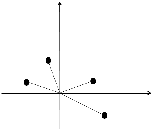
To get some insight into how we should solve this problem, let’s suppose we have an extremely simple set of training data. We’ll suppose a human operator has ranked three documents $d_1, d_2, d_3$ for just a single query $q$ . Of course, real training data will need to involve many more documents and queries, but we can learn a lot by starting with this. We have three feature vectors for these three cases, $\vec \psi(q,d_1), \vec \psi(q,d_2), \vec \psi(q,d_3)$ . I’ve illustrated these in the following diagram – to avoid clutter, rather than write $\vec \psi(q,d_j)$ repeatedly in the diagram, I’ve labelled each vector simply by its document number, $d_j$ , as well as (in parentheses) by its order of relevance as ranked by a human operator:

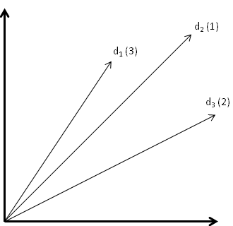
There are a few reasonable observations:

If a feature vector $\vec \psi(q,d)$ is up and to the right of $\vec \psi(q,d')$ then it’s better along both axes (PageRank and cosine similarity). It seems reasonable to conclude that $d$ is a better result than $d'$ .
Coversely, if $\vec \psi(q,d)$ is down and to the left of $\vec \psi(q,d')$ then $d$ should always be ranked below $d'$ .
The hard cases are when $\vec \psi(q,d)$ is up and to the left of $\vec \psi(q,d')$ , or down and to the right, in which case it’s not entirely clear

Note, by the way, that I don’t want to claim that that these observations are “proveable” in any way: they’re just reasonable observations, at least for the particular features (cosine similarity and PageRank) that we’re using. The idea here is simply to figure out some reasonable heuristics which we will eventually combine to suggest an algorithm for learning how to rank webpages.

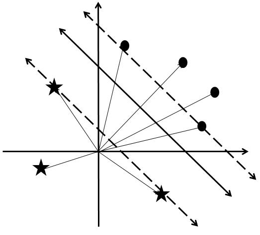
With the observations above as motivation we’ll adopt the heuristic that it is the vector of feature differences $\vec \phi(q,d,d') := \vec \psi(q,d)-\vec \psi(q,d')$ that determines whether $d$ should be ranked above $d'$ , or vice versa. In other words, we’re going to require that the relative ranking of $d$ and $d'$ is a function of the components of $\vec \phi(q,d,d')$ , and not of either individual feature vector alone. So the problem now becomes: how should we use $\vec \phi(q,d,d')$ to rank $d$ and $d'$ ? A clue is provided by looking at the vectors of feature differences for our training data:

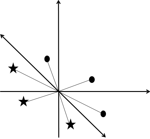
I haven’t labelled the vectors explicitly with $q, d$ and $d'$ , but it’s pretty easy to figure out which is which, if you look carefully. Instead, I’ve labelled each feature difference vector $\vec \phi(q,d,d')$ with a filled in oval when $d$ is ranked better than $d'$ , and with a star when $d'$ is ranked better than $d$ . Examining the vectors carefully, we see that the vectors with an oval all “point the same way” as one another, while the vectors with a star also all point the same way as one another, but in the opposite direction. We can make this intuition more precise by saying that the two sets of vectors are separated into two half-spaces by a line:

So one way we could determine whether a feature difference vector is labelled by an oval or a cross is simply by determining which half-space it is in, i.e., by determing which side of the line it’s on. Or to reformulate it in our original terms: we can tell whether a webpage $d$ ranks higher than a webpage $d'$ simply by determining which half-space the feature difference vector $\vec \phi(q,d,d')$ is in.

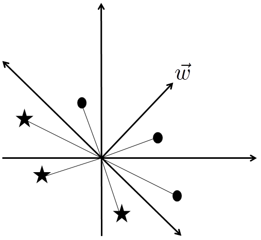
In higher-dimensional feature spaces this idea generalizes to separating the feature difference vectors into two half-spaces which are on opposite sides of a separating hyperplane. A convenient way of specifying this separating hyperplane, in any number of dimensions, is to introduce a normal vector $\vec w$ to the hyperplane. I’ve illustrated such a normal vector below for two dimensions, but you should imagine that we’re working in higher dimensions:

The condition for a feature difference vector to be in (say) the upper half-space is that $\vec \phi(q,d,d') \cdot \vec w > 0$ . To be in the lower half-space the condition is that $\vec \phi(q,d,d') \cdot \vec w < 0[/latex]. Summing everything up, we can check whether the document [latex]d[/latex] should be ranked above or below [latex]d'[/latex] simply by computing the sign of [latex]\vec \phi(q,d,d') \cdot \vec w[/latex]. The above observations suggest an algorithm for using the feature difference vectors to determine search relevance. It's a pretty obvious generalization of what I've just described, but at the risk of repeating myself I'll write it all out explicitly. To start, we assume that a set of training data has been provided by human operators. Those operators have been given a set of training queries [latex]q_1,q_2,\ldots,q_m[/latex] and training documents [latex]d_1,d_2,\ldots,d_n[/latex]. For each training query they've ranked each training document in order of relevance to that query. They might decide, for example, that for the query [latex]q_1[/latex], the document [latex]d_{17}[/latex] should be the top-ranked query, [latex]d_5[/latex] the second-ranked query, and so on. This training data provides us with a whole lot of feature difference vectors [latex]\vec \phi(q_i,d_j,d_k)[/latex]. These vectors can be divided up into two sets. The first set, which we'll call training data set [latex]A[/latex], contains those feature difference vectors for which [latex]d_j[/latex] has been ranked more highly than [latex]d_k[/latex]. The second set, which we'll call training data set [latex]B[/latex], contains those feature difference vectors for which [latex]d_k[/latex] has been ranked more highly than [latex]d_j[/latex]. We then find a separating hyperplane that separates these two data sets, i.e., with the <em>upper half-space</em> containing data set [latex]A$ (where $d_j$ is ranked more highly than $d_k$ for $q_i$ ), and a lower half-space containing data set $B$ .

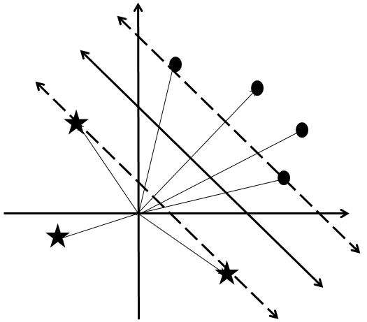
Suppose now that $q$ is any query – not necessarily a training query. And suppose $d$ and $d'$ are any two documents, not just training documents. We rank $d$ above $d'$ for query $q$ if the feature difference vector $\vec \phi(q,d,d')$ lies in the upper half-space. And we rank $d$ below $d'$ if it lies in the lower half-space. This completes the description of the algorithm.

There are many problems with this basic algorithm. One problem becomes evident by going back to our primitive training data and adding an extra document:

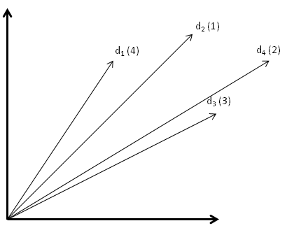
Inspecting the feature difference vectors reveals a problem:

I’ve simplified the picture by showing only the feature difference vectors $\phi(q,d,d')$ in data set $A$ , i.e., those for which $d$ ranks more highly than $d'$ ; data set $B$ contains the negation of those vectors. It should be clear that there is no half-space which can be used to divide up the vectors into two sets. It’s not geometrically possible. The way we’ll deal with this is by modifying the algorithm in such a way as to find a half-space which approximately divides the two sets of feature difference vectors into half-spaces. I’ll explain how to do this approximate division later in the post.

Before getting to the approximate division, though, we’ll warm up by figuring out much more explicitly how to do the division into two half-spaces when it is possible. It’s all very well for me to glibly say that we should “figure out which half-space the vector $\phi(q,d,d')$ is in”, but how can we actually do this in practice? In the next section I’ll introduce support vector machines, which are a way of doing this kind of division explicitly. Once we’ve understood the basics of support vector machines, we’ll come back to the question of how to divide two sets of vectors into approximate half-spaces.

Problems

Suppose the basic algorithm that I’ve described works, i.e., a division into half-spaces is possible. Suppose that for a particular query $q$ the document $d$ is ranked above $d'$ and $d'$ is ranked above $d''$ . Prove that the algorithm will rank $d$ above $d''$ .

Support vector machines

Support vector machines are a technique for partitioning two sets of vectors (data set $A$ and data set $B$ ) into half-spaces separated by a separating hyperplane. The technique is guaranteed to work whenever such a partitioning is possible, and whatsmore the partitioning is optimal, in a sense I’ll make precise. In this section I’ll describe briefly how support vector machines work.

As an aside, you’ll note that the notion of search (and related topics) wasn’t mentioned anywhere in the last paragraph. That’s because support vector machines aren’t about search. Instead, they’re a general technique for dividing sets of vectors into half-spaces, a technique which can be applied to many different problems in machine learning and artificial intelligence, not just search. So support vector machines are a useful technique to understand, even if you’re not especially interested in search. End of aside.

A priori if someone just gives you two sets of vectors, $A$ and $B$ , it’s not always going to be clear whether a partitioning into two half-spaces is possible. But let’s assume that such a partitioning is possible, and we’ll return later to what happens when it’s not. What we’d like to do is to find an explicit way of specifying a separating hyperplane:

Note that in the last section our separating hyperplanes passed through the origin. But for support vector machines we’ll also allow hyperplanes which don’t pass through the origin. One way to explicitly specify such a hyperplane is as the set of vectors $\vec x$ satisfying the equation:

$\vec w \cdot \vec x + b = 0,$

where $\vec w$ is a vector normal to the separating hyperplane, and $b$ is a constant. Together, $\vec w$ and $b$ specify the hyperplane. The goal of the support vector machine is to take data sets $A$ and $B$ , and use them to construct values for $\vec w$ and $b$ which specify a separating hyperplane. Whatsmore, we’ll try to do this in such a way that we maximize the size of the “wedge” between the two data sets,

where we require that the two edges of the wedge (called support or supporting hyperplanes) be parallel to the separating hyperplane itself. In other words, the goal is to choose the separating hyperplane (i.e., to choose $\vec w$ and $b$ ) in such a way that these two supporting hyperplanes are as far apart from one another as possible.

Let me mention, by the way, that I’m not mad keen on the notations we’ve been using, such as $\vec w$ and $b$ . Unfortunately, it’s not going to get any better – we have some $\xi$ ‘s and $C$ ‘s in our near future, and I’m sorry to say that the origin of those notations won’t be much more transparent than the origins of $\vec w$ and $b$ . I’m using what seems to be standard notation in the support vector machine literature, but it’s not very good notation, in my opinion: it has little or no mnemonic value, and is very non-uniform to boot. While I’m complaining, I’ll mention one more thing: the vector $\vec w$ is sometimes known as the weight vector, again, for reasons which seem obscure. End of rant.

Let’s get back to the problem of choosing $\vec w$ and $b$ so that the two supporting hyperplanes are as far apart from one another as possible. To do that, we need to figure out a way of expressing the distance between the two supporting hyperplanes in terms of $\vec w$ and $b$ . Without any loss of generality, we’ll suppose that the separating hyperplane is halfway between the two supporting hyperplanes:

Let’s fix our attention on one of the two supporting hyperplanes, say, the one that is “higher up” in the picture above. We’ll suppose, also without any loss of generality, that this is the hyperplane supporting data set $A$ . By rescaling $\vec w$ and $b$ if necessary, we can ensure that this support hyperplane has the equation

$\vec w \cdot \vec x + b = 1,$

and so the constraint that this hyperplane support data set $A$ may be expressed as $\vec w \cdot \vec x + b \geq 1$ . This is an important constraint: it’s the constraint on data set $A$ .

Exercises

If you’re not comfortable with hyperplanes you may not immediately see why the kind of rescaling of $\vec w$ and $b$ which I did in the last paragraph is always possible. If this is the case, then write out an explicit proof.

We can now determine the distance between the supporting and separating hyperplane by introducing a vector $\Delta$ which is: (a) normal to both hyperplanes, and (b) connects the two hyperplanes. A bit more precisely, $\vec \Delta := \vec x'-\vec x$ , where $\vec x'$ is in the supporting hyperplane and $\vec x$ is the projection of $\vec x'$ onto the separating hyperplane:

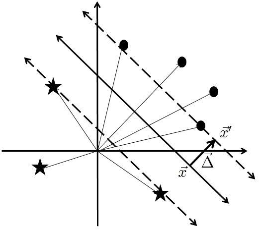
Our goal is to find the length of $\vec \Delta$ . Taking the difference of the equations $\vec w \cdot \vec x' + b = 1$ and $\vec w \cdot \vec x + b = 0$ , we have $\vec w \cdot \vec \Delta = 1$ . Since $\vec \Delta$ and $\vec w$ are both normal to the separating hyperplane, and thus parallel, it follows that $\Delta w = 1$ , where I am omitting the $\vec \cdot$ in order to denote length. It follows that the distance from the separating to the supporting hyperplane is $\Delta = 1/w$ .

We chose the separating hyperplane to be halfway between the two supporting hyperplanes, and so the total size of the wedge is $2\Delta = 2/w$ . As a result, maximizing the size of the wedge is equivalent to maximizing $2/w$ . This is subject to the constraint on data set $A$ , namely that $\vec w \cdot \vec x_j + b \geq 1$ for all the vectors $\vec x_j$ in data set $A$ . There’s also a similar constraint for data set $B$ ,

$\vec w \cdot \vec x_j + b \leq -1$

for all the vectors $\vec x_j$ in data set $B$ . The supporting hyperplane for data set $B$ satisfies this condition with equality.

Exercises

Prove that $\vec w \cdot x + b = -1$ is the equation for the supporting hyperplane for data set $B$ .

There is a reasonably nice way of combining the two sets of constraint inequalities for data sets $A$ and $B$ . That’s to label each vector $\vec x_j$ with a value $y_j = +1$ if $\vec x_j$ is in data set $A$ , and with $y_j = -1$ if $\vec x_j$ is in data set $B$ . With these labels, we can now express the constraints on $\vec w$ and $b$ in a single set of inequalities

$y_j (\vec w \cdot \vec x_j + b) \geq 1,$

with equality holding if the vector in question is on a supporting hyperlane (a so-called support vector). This single set of inequalities represents the constraint that $\vec w$ and $b$ really do define separating and supporting hyperplanes for data sets $A$ and $B$ , and that the distance between the supporting hyperplanes is $2/w$ .

Rather than maximize $2/w$ subject to the above constraints, it’s conventional to instead minimize $w^2/2 = \vec w \cdot \vec w /2$ , subject to the same constraints. This is obviously equivalent, and the reason we make this change will become clear shortly.

Summing up, our problem is to find $\vec w$ and $b$ which minimize the value of:

$\frac{w^2}{2}$

subject to the constraints

$y_j (\vec w \cdot \vec x_j + b) \geq 1,$

where $y_j = +1$ if $\vec x_j$ is in data set $A$ , and $y_j = -1$ if $\vec x_j$ is in data set $B$ .

This formulation of our problem represents real progress. The reason is that the problem just described is an instance of a very well-known type of problem in mathematics and computer science, called a quadratic programming problem. Although quadratic programs don’t in general have simple, closed-form solutions, they’ve been studied for decades and are well understood, and there are good algorithms and libraries for solving them. It’s because quadratic programs are so well understood that we changed from maximizing $2/w$ to minimizing $w^2/2$ (the $1/2$ is conventional, since it simplifies certain other expressions in the theory of quadratic programming). Indeed, quadratic programs are so well understood that not only are there many libraries for solving quadratic programs, some of those libraries have been specially designed to solve the quadratic programs which arise from support vector machines. Here’s a rather lengthy list of libraries and packages which are designed for support vector machines, and you may wish to experiment with those libraries.

Incidentally, one potentially confusing thing about the quadratic programming problem posed above – and one of the reasons I complain about the notation – is to be clear on exactly what is being solved for. The $y_j$ and $\vec x_j$ are known input data, which should be regarded as fixed, and the task is to solve for $\vec w$ and $b$ . This is obviously rather different from the traditional use of $x$ and $y$ to denote what we’re solving for, and it’s good to keep this clearly in mind.

We can now explain what a support vector machine actually is. We have some problem – like the search ranking problem – which generate sets of training data, $A$ and $B$ , in a vector space. The support vector machine will find the parameters $\vec w$ and $b$ for the separating hyperplane, so that the “wedge” between these two data sets is maximized, i.e., the distance between the supporting hyperplanes is maximized. We can then use the parameters $\vec w$ and $b$ to classify new problem instances $\vec x$ as being of type $A$ or type $B$ . In particular, we classify $\vec x$ as being of type $A$ if $\vec w \cdot \vec x + b \geq 0$ , and of type $B$ if $\vec w \cdot \vec x + b < 0[/latex]. A support vector machine is an example of a <a href="http://en.wikipedia.org/wiki/Linear_classifier">linear classifier</a>: a decision procedure which makes a classification decision (``Is page [latex]d$ ranked higher than page $d'$ “) using some linear function of the feature vector describing the problem instance. It’s a binary linear classifier, since the classification is into two types. Such classifiers are useful because they have such generality. Have a bunch of photos, and want to classify which are photos of fish? Spend some time (or money) generating training data, and some more time coming up with a few features that seem like they might be helpful. Then find a support vector machine which can be used to classify more problem instances, and see how well it works! Of course, nothing guarantees that it’ll work well, but with good feature selection it seems that if often really does work well in practice.

I won’t go any deeper into the theory or practice of support vector machines in this post. Instead, we’ll return to the question of how to deal with the fact that sometimes it’s not possible to separate the training data into two half-spaces. What we’ll see is that it is possible to do an approximate separation, using the same techniques of quadratic programming. This is known as a support vector machine with a soft margin. Once we’ve understood how that works I’ll come back to what this all means in the context of search.

Support vector machines with a soft margin

In our earlier discussion of search, we saw an example where the feature difference vectors in a set of training data cannot be partitioned into two half-spaces (again, as earlier, this diagram only shows feature difference vectors $\vec \phi(q,d,d')$ where $d$ should be ranked higher than $d'$ , i.e., it shows only data set $A$ ):

What can we do in this situation? There is a way of modifying the support vector machine idea to find an approximate way of partitioning two sets of vectors into half-spaces. The idea is to allow some of the vectors to slightly violate the half-space constraints. We compensate for these violations by paying a penalty in the function being minimized. This will ensure that any violations are quite small.

The way this idea is implemented is as follows. We introduce some slack variables $\xi_j$ , one for each vector $\vec x_j$ . The size of the slack variable $\xi_j$ will determine how much violation of the half-space constraint is allowed for the vector $\vec x_j$ . In particular, the constraints on the vectors are now relaxed to be

$y_j (\vec w \cdot \vec x_j + b) \geq 1-\xi_j.$

We also impose the constraint on the slack variables that

$\xi_j \geq 0,$

simply so as to ensure that we’re not over-constraining our vectors by picking a negative value for $\xi_j$ . The larger a given $\xi_j$ the more the vector $\vec x_j$ can violate the partitioning into half-spaces. For that reason we introduce a new term in the function we want to minimize, in order to penalize excursions from the half-space:

$\frac{w^2}{2} + C \sum_j \xi_j.$

Here $C > 0$ is called the soft margin parameter. If $C$ is large, then we pay a substantial penalty even for small excursions from the half-spaces. On the other hand, if $C$ is small then we pay only a small penalty, and so we can expect larger excursions from the half-spaces.

The problem defined in the last paragraph is (again) a quadratic program, and standard algorithms and libraries can be used to solve the program. Also as in the last section, given a solution to the program we can use that solution as a binary linear classifier. In particular, suppose $\vec w$ and $b$ appear in such a solution. Then given a new problem instance $\vec x$ to be classified, we classify it as being of type $A$ if $\vec w \cdot \vec x + b \geq 0$ , and of type $B$ if $\vec w \cdot \vec x + b < 0[/latex]. An issue that I haven't addressed - and don't yet know how to solve - is how to choose the soft margin parameter, [latex]C[/latex]. As a starting point for understanding this choice, let me at least state the following: <strong>Theorem:</strong> A solution to the quadratic program above always exists. This is a major improvement over the situation without the soft margin, where it's not even guaranteed that a solution will exist. It means that no matter what the training data or soft margin parameter, we can always build a binary linear classifier using the support vector machine with that soft margin. I won't give the proof of the theorem, but the intuition is simple enough: for any choice of [latex]\vec w$ and $b$ , by choosing $\xi_j$ sufficiently large we can ensure that $\vec x_j$ satisfies the constraints. A fairly standard continuity and compactness argument should do the trick (modulo some reasonable assumptions, e.g., that we’re working in finite dimensions and with finite data sets).

While the theorem above is an encouraging start, it’s not what we really want. What we’d like is to understand how best to choose $C$ . Ideally, this means understanding how different choices of $C$ impact the solutions which are found, and being more precise about what sorts of excursions from the half-spaces we are willing to allow, and what impact this has on the quality of classifications. This is, obviously, a challenging theoretical program! However, for the very practical problem of combining different relevancy factors in search, I think a great deal of progress could be made simply by trying out different values of $C$ , and testing to see which value empirically gives the best results. Trial-and-error is often better than being smart.

Problems

Above, I talked about the soft margin parameter $C$ being “large” or “small”, but didn’t explain exactly what I meant. How could we make these notions more precise?
Suppose the data sets have the property that data set $A$ is the negation of data set $B$ , i.e., for each vector $\vec x$ in $A$ , there is a corresponding vector $-\vec x$ in $B$ , and vice versa. (This is the case in the search problem, for example.) Prove that if a value for $b$ appears in a solution to the quadratic program, then there is also a solution to the quadratic program with value $-b$ . In fact, it’s possible to prove (though we won’t do so) that the solution to the quadratic program is unique, and so we must have $b=-b$ , and therefore $b=0$ . It follows that for the search problem we can assume $b=0$ in the solution to the quadratic program.

Problems for the author

The modifications to the support vector machine model made in this section are quite ad hoc. In particular, choosing the penalty to be $C \sum_j \xi_j$ seems to me to be quite unmotivated. Is there some natural geometric way of deriving this model? Even better, is there a principled way of deriving the model?

Search revisited

Let’s return to the problem of search. As we saw in the last section, we can use training data to build a support vector machine (with soft margin) that, given a query, $q$ , will tell us whether a document $d$ is more relevant than $d'$ , or vice versa. Of course, this ranking decision won’t in any sense be “provably” optimal – it’s not even clear what that would mean, exactly. But the support vector machine has the advantage that it takes into account all the different relevancy information we have (all the different features), and it does so in a way that reflects the training data.

Problems

Suppose that the relevancy ranking algorithm just described ranks the document $d$ above $d'$ , and $d'$ is ranked above $d''$ , for some query $q$ . Prove that it will also rank $d$ above $d''$ .

How can we use this support vector machine in practice? One way is as follows. Suppose we have $n$ documents. A user enters a query $q$ . Then because we can easily compare any two documents in the collection, we can use a sort algorithm such as quicksort to produce a rank ordering of the $n$ documents, using $O(n \log n)$ comparisons.

This approach isn’t really the best, though. Suppose, for comparison, that you had $n$ documents and wanted to figure out the top $10$ documents (say), as ranked by PageRank. You could do a single pass over all $n$ documents, keeping a running tally of the best $10$ documents found to date. That’d take $O(n)$ running time, which is significantly faster.

Of course, we can apply the same idea with our support vector machine. Simply do a single pass over all $n$ documents, maintaining a running tally of the best $10$ documents found to date. More precisely, each time you examine a new document, simply compare it to the current list of the top $10$ documents, using the support vector machine, and if the new document is better than any of those, update the list.

Quite aside from being significantly faster than ranking all documents, a major advantage of the running tally method is that it is easily run on a large cluster. Each machine simply computes the top $10$ documents stored on that machine, and then those short lists are merged at a central location.

This post has introduced a simple technique which can be used to combine different notions of search relevancy. It’s very much an introduction, and there are a huge number of problems I have not addressed. Perhaps the biggest one is this: how well does this procedure work in practice? That is, does it give a satisfying search experience, one which is significantly improved by the addition of new relevancy factors? I’d love to test this out, but I don’t have good enough trial data (yet) to do a really good test. Maybe someone can point to some real data along these lines.

At this point in the original drafting of this post, I began enumerating problems one might want to think about in applying these ideas to improve a real search engine. The list quickly became very long: there’s a lot to think about! So rather than list all those problems, I’ll conclude with just a couple of problems which you may ponder. Enjoy!

Problems for the author

Suppose we’re running a real-life search engine, and were thinking of introducing an additional feature. How could we use A/B testing to determine whether or not that additional feature does a little or a lot to help improve relevancy ranking?
At the beginning of this post I proposed figuring out (by thinking hard!) a principled way of combining cosine similarity and PageRank to come up with a composite measure of relevance. Find such a principled way of making the combination. I expect that the value in attacking this problem will lie not so much in whatever explicit combination I find, but rather in better understanding how to make such combinations. It may also shed some light on when we expect the machine learning approach to work well, and when we’d expect it to work poorly.

Interested in more? Please follow me on Twitter. You may also enjoy reading my new book about open science, Reinventing Discovery.

3 comments

Jochen Wersdörfer says:

February 4, 2012 at 1:31 pm

Since you asked for trial data, here’s the website of the 2010 yahoo learning to rank challenge:

http://learningtorankchallenge.yahoo.com/

The datasets are quite big and are said to come from a real web search engine :). Unfortunately no description of the features (>500) is provided.

http://research.microsoft.com/en-us/projects/mslr/default.aspx

Microsoft even shared a description of the features.

Skimming your article only, i wondered how you combine the SVM-scores into an explicit ranking? I played around with pairwise ranking myself and decided to sum the scores for the n(n -1) / 2 pairs. Which works okish, but is still an ugly heuristic…
1. Michael Nielsen says:
  
  February 6, 2012 at 4:59 pm
  
  Thanks for the pointers, I’ll take a look!
  
  As regards your explicit ranking question, take a look at the next post, which is quite a bit clearer on this question.
Pingback: Addendum on search and support vector machines | DDI

Comments are closed.