In this post I explain how to compute PageRank using the MapReduce approach to parallelization. This gives us a way of computing PageRank that can in principle be automatically parallelized, and so potentially scaled up to very large link graphs, i.e., to very large collections of webpages. In this post I describe a single-machine implementation which easily handles a million or so pages. In future posts we’ll use a cluster to scale out much further – it’ll be interesting to see how far we can get.
I’ve discussed PageRank and MapReduce at length in earlier posts – see here for MapReduce, and here and here for PageRank – so in this post we’ll just quickly review the basic facts. Let’s start with PageRank. The idea is that we number webpages [tex]0,\ldots,n-1[/tex]. For webpage number [tex]j[/tex] there is an associated PageRank [tex]q_j[/tex] which measures the importance of page [tex]j[/tex]. The vector [tex]q = (q_0,\ldots,q_{n-1})[/tex] of PageRanks is a probability distribution, i.e., the PageRanks are numbers between [tex]0[/tex] and [tex]1[/tex], and sum up to one, in total. The PageRank [tex]q_j[/tex] measures the importance of page [tex]j[/tex]; the bigger the PageRank, the more important the page.
How is the PageRank vector [tex]q[/tex] computed? I’ll just describe the mathematical upshot here; the full motivation in terms of a crazy websurfer who randomly surfs the web is described in an earlier post. The upshot is that the PageRank vector [tex]q[/tex] can be defined by the equation (explanation below):
[tex] q \leftarrow M^j P. [/tex]
What this equation represents is a starting distribution [tex]P[/tex] for the crazy websurfer, and then [tex]j[/tex] steps of “surfing”, with each action of [tex]M[/tex] representing how the distribution changes in a single step. [tex]P[/tex] is an [tex]n[/tex]-dimensional vector, and [tex]M[/tex] is an [tex]n \times n[/tex] matrix whose entries reflect the link structure of the web in a way I’ll make precide below. The PageRank [tex]q[/tex] is defined in the limit of large [tex]j[/tex] – in our examples, convergence typically occurs for [tex]j[/tex] in the range [tex]10[/tex] to [tex]30[/tex]. You might wonder how [tex]P[/tex] is chosen, but part of the magic of PageRank is that it doesn’t matter how [tex]P[/tex] is chosen, provided it’s a probability distribution. The intuition is that the starting distribution for the websurfer doesn’t matter to the websurfer’s long-run behaviour. We’ll start with the uniform probability distribution, [tex]P = (1/n,1/n,\ldots)[/tex], since it’s easy to generate.
How is the matrix [tex]M[/tex] defined? It can be broken up into three pieces
[tex] M = s A + s D + t E, [/tex]
including: a contribution [tex]sA[/tex] representing the crazy websurfer randomly picking links to follow; a contribution [tex]sD[/tex] due to the fact that the websurfer can’t randomly pick a link when they hit a dangling page (i.e., one with no outbound links), and so something else needs to be done in that case; and finally a contribution [tex]tE[/tex] representing the websurfer getting bored and “teleporting” to a random webpage.
We’ll set [tex]s = 0.85[/tex] and [tex]t = 1-s = 0.15[/tex] as the respective probabilities for randomly selecting a link and teleporting. See this post for a discussion of the reasons for this choice.
The matrix [tex]A[/tex] describes the crazy websurfer’s linkfollowing behaviour, and so, in some sense, encodes the link structure of the web. In particular, suppose we define [tex]\#(j)[/tex] to be the number of links outbound from page [tex]j[/tex]. Then [tex]A_{kj}[/tex] is defined to be [tex]0[/tex] if page [tex]j[/tex] does not link to page [tex]k[/tex], and [tex]1/\#(j)[/tex] if page [tex]j[/tex] does link to page [tex]k[/tex]. Stated another way, the entries of the [tex]j[/tex]th column of [tex]A[/tex] are zero, except at locations corresponding to outgoing links, where they are [tex]1/\#(j)[/tex]. The intuition is that [tex]A[/tex] describes the action of a websurfer at page [tex]j[/tex] randomly choosing an outgoing link.
The matrix [tex]D[/tex] is included to deal with dangling pages, i.e., pages with no outgoing links. For such pages it is obviously ambiguous what it means to choose an outgoing link at random. The conventional resolution is to choose another page uniformly at random from the entire set of pages. What this means is that if [tex]j[/tex] is a dangling page, then the [tex]j[/tex]th column of [tex]D[/tex] should have all its entries [tex]1/n[/tex], otherwise, if [tex]j[/tex] is not dangling, all the entries should be zero. A compact way of writing this is
[tex] D = e d^T/ n, [/tex]
where [tex]d[/tex] is the vector of dangling pages, i.e., the [tex]j[/tex]th entry of [tex]d[/tex] is [tex]1[/tex] if page [tex]j[/tex] is dangling, and otherwise is zero. [tex]e[/tex] is the vector whose entries are all [tex]1[/tex]s.
The final piece of [tex]M[/tex] is the matrix [tex]E[/tex], describing the bored websurfer teleporting somewhere else at random. This matrix has entries [tex]1/n[/tex] everywhere, representing a uniform probability of going to another webpage.
Okay, that’s PageRank in a mathematical nutshell. What about MapReduce? Again, I’ll just remind you of the basic details – if you want an introduction, see this post. MapReduce is one of those ideas where understanding is really helped by first working through an example, rather than starting with an abstract description, like I’m about to give, so if you’re not familiar with MapReduce, I strongly suggest reading the earlier post.
The input to a MapReduce job is a set of (input_key,input_value) pairs. Each pair is used as input to a function mapper(input_key,input_value) which produces as output a list of intermediate keys and intermediate values:
[(intermediate_key,intermediate_value),
 (intermediate_key',intermediate_value'),
 ...]
The output from all the different input pairs is then sorted, so that intermediate values associated with the same intermediate_key are grouped together in a list of intermediate values. The reducer(intermediate_key,intermediate_value_list) function is then applied to each intermediate key and list of intermediate values, to produce the output from the MapReduce job.
Computing PageRank with MapReduce
Okay, so how can we compute PageRank using MapReduce? The approach we’ll take is to use MapReduce to repeatedly multiply a vector by the matrix [tex]M[/tex]. In particular, we’re going to show that if [tex]p[/tex] is a probability distribution, then we can easily compute [tex]Mp[/tex] using MapReduce. We can thus compute [tex]M^jP[/tex] using repeated invocations of MapReduce. Those invocations have to be done serially, but the individual MapReduce jobs are themselves all easily parallelized, and so we can potentially get a speedup by running those jobs on a big cluster. Much more about doing that in later posts.
The nub of the problem, then, is figuring out how to compute [tex]Mp[/tex], given a starting probability distribution [tex]p[/tex]. Let’s start out with a rough approach that gets the basic idea right, essentially using MapReduce to compute [tex]Ap[/tex]. We’ll see below that it’s easy to fix this up to take dangling nodes and teleportation into account. The fix involves introducing an additional MapReduce job, though, so each multiplication step [tex]p \rightarrow Mp[/tex] actually involves two MapReduce jobs, not just one. For now, though, let’s concentrate on roughing out a MapReduce job that computes [tex]Ap[/tex].
As input to the MapReduce computation, we’ll use (key,value) pairs where the key is just the number of the webpage, let’s call it j, and value contains several items of data describing the page, including [tex]p_j[/tex], the number [tex]\#(j)[/tex] of outbound webpages, and a list [k_1,k_2,...] of pages that j links to.
For each of the pages k_l that j links to, the mapper outputs an intermediate key-value pair, with the intermediate key being k_l and the value just the contribution [tex]p_j/\#(j)[/tex] made to the PageRank. Intuitively, this corresponds to the crazy websurfer randomly moving to page k_l, with the probability [tex]p_j/\#(j)[/tex] combining both the probability [tex]p_j[/tex] that they start at page [tex]j[/tex], and the probability [tex]p_j/\#(j)[/tex] that they move to page k_l.
Between the map and reduce phases, MapReduce collects up all intermediate values corresponding to any given intermediate key, k, i.e., the list of all the probabilities of moving to page k. The reducer simply sums up all those probabilities, outputting the result as the second entry in the pair (k,p_k'), and giving us the entries of [tex]Ap[/tex], as was desired.
To modify this so it computes [tex]Mp[/tex] we need to make three changes.
The first change is to make sure we deal properly with dangling pages, i.e., we include the term [tex]sD[/tex]. One possible way is to treat dangling pages as though they have outgoing links to every single other page, [0,1,2,...]. While this works, it would require us to maintain many very large lists of links, and would be extremely inefficient.
A better way to go is to use our earlier expression [tex]D = e d^T/n[/tex], and thus [tex]Dp = e (d\cdot p)/n[/tex], where [tex]d \cdot p[/tex] is the inner product between the vector [tex]d[/tex] of dangling pages, and [tex]p[/tex]. Computing [tex]Dp[/tex] then really boils down to computing [tex]d \cdot p[/tex].
We can compute [tex]d \cdot p[/tex] using a separate MapReduce job which we run first. This job computes the inner product, and then passes it as a parameter to the second MapReduce job, which is based on the earlier rough description, and which finishes off the computation. This first MapReduce job uses the same input as the earlier job – a set of keys j corresponding to pages, and values describing the pages, i.e., containing the value for p_j, and a description of the outbound links from page j. If page j is dangling the mapper outputs the intermediate pair (1,p_j), otherwise it outputs nothing. All the intermediate keys are the same, so the reducer acts on just one big list, summing up all the values p_j for dangling pages, giving us the inner product we wanted.
As an aside, while this prescription for computing the inner product using MapReduce is obviously correct, you might worry about the fact that all the intermediate keys have the same value. This means all the intermediate values will go to a single reducer, running on just one machine in the cluster. If there are a lot of dangling pages, that means a lot of communication and computation overhead associated with that single machine – it doesn’t seem like a very parallel solution. There’s actually a simple solution to this problem, which is to modify the MapReduce framework just a little, introducing a “combine” phase inbetween map and reduce, which essentially runs little “mini-reducers” directly on the output from all the mappers, offloading some of the reduce functionality onto the machines used as mappers. We won’t explore this idea in detail here, but we will implement it in future posts, and we’ll see that in practice having just a single key isn’t a bottleneck.
The second change we need to make in our rough MapReduce job is to include the teleportation step. This can be done easily by modifying the reducer to include a contribution from teleportation.
The third change we need to make in our rough MapReduce job is somewhat subtle; I actually didn’t realize I needed to make this change until after I ran the code, and realized I had a bug. Think about the set of intermediate keys produced by the mappers. The only way a given page can appear as an intermediate key is if it’s linked to by some other page. Pages with no links to them won’t appear in the list of intermediate keys, and so won’t appear in the output from the MapReduce job. The way we deal with this problem is by modifying the mapper so that it emits one extra key-value pair as output. Namely, if it takes as input (j,value), then it emits all the intermediate keys and values described earlier, and an additional pair (j,0), which represents a probability [tex]0[/tex] of moving to page j. This ensures that every page j will appear in the list of intermediate keys, but doesn’t have any impact on the probability of moving to page j; you can think of it simply as a placeholder output.
That completes the high-level theoretical description of computing PageRank using MapReduce. In the next section of the post I’ll describe a simple Python implementation of this MapReduce-based approach to PageRank. If you’re not interested in the implementation, you can skip to the final section, where I talk about how to think about programming with MapReduce – general heuristics you can use to put problems into a form where MapReduce can be used to attack them.
Implementation
The Python code to implement the above PageRank algorithm is straightforward. To run it on just a single machine we can use the exact same MapReduce module I described in my earlier post; for convenience, here’s the code:
# map_reduce.py
# Defines a single function, map_reduce, which takes an input
# dictionary i and applies the user-defined function mapper to each
# (input_key,input_value) pair, producing a list of intermediate
# keys and intermediate values.  Repeated intermediate keys then
# have their values grouped into a list, and the user-defined
# function reducer is applied to the intermediate key and list of
# intermediate values.  The results are returned as a list.

import itertools

def map_reduce(i,mapper,reducer):
  intermediate = []
  for (key,value) in i.items():
    intermediate.extend(mapper(key,value))
  groups = {}
  for key, group in itertools.groupby(sorted(intermediate),
                                      lambda x: x[0]):
    groups[key] = list([y for x, y in group])
  return [reducer(intermediate_key,groups[intermediate_key])
          for intermediate_key in groups]
With that code put in a file somewhere your Python interpreter can find it, here’s the code implementing PageRank:
# pagerank_mr.py
#
# Computes PageRank, using a simple MapReduce library.
#
# MapReduce is used in two separate ways: (1) to compute
# the inner product between the vector of dangling pages
# (i.e., pages with no outbound links) and the current
# estimated PageRank vector; and (2) to actually carry
# out the update of the estimated PageRank vector.
#
# For a web of one million webpages the program consumes
# about one gig of RAM, and takes an hour or so to run,
# on a (slow) laptop with 3 gig of RAM, running Vista and
# Python 2.5.
import map_reduce
import numpy.random
import random
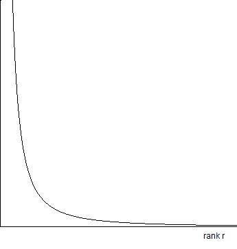
def paretosample(n,power=2.0):
# Returns a sample from a truncated Pareto distribution
# with probability mass function p(l) proportional to
# 1/l^power. The distribution is truncated at l = n.
m = n+1
while m > n: m = numpy.random.zipf(power)
return m
def initialize(n,power):
# Returns a Python dictionary representing a web
# with n pages, and where each page k is linked to by
# L_k random other pages. The L_k are independent and
# identically distributed random variables with a
# shifted and truncated Pareto probability mass function
# p(l) proportional to 1/(l+1)^power.
# The representation used is a Python dictionary with
# keys 0 through n-1 representing the different pages.
# i[j][0] is the estimated PageRank, initially set at 1/n,
# i[j][1] the number of outlinks, and i[j][2] a list of
# the outlinks.
# This dictionary is used to supply (key,value) pairs to
# both mapper tasks defined below.
# initialize the dictionary
i = {}
for j in xrange(n): i[j] = [1.0/n,0,[]]
# For each page, generate inlinks according to the Pareto
# distribution. Note that this is somewhat tedious, because
# the Pareto distribution governs inlinks, NOT outlinks,
# which is what our representation is adapted to represent.
# A smarter representation would give easy
# access to both, while remaining memory efficient.
for k in xrange(n):
lk = paretosample(n+1,power)-1
values = random.sample(xrange(n),lk)
for j in values:
i[j][1] += 1 # increment the outlink count for page j
i[j][2].append(k) # insert the link from j to k
return i
def ip_mapper(input_key,input_value):
# The mapper used to compute the inner product between
# the vector of dangling pages and the current estimated
# PageRank. The input is a key describing a webpage, and
# the corresponding data, including the estimated pagerank.
# The mapper returns [(1,pagerank)] if the page is dangling,
# and otherwise returns nothing.
if input_value[1] == 0: return [(1,input_value[0])]
else: return []
def ip_reducer(input_key,input_value_list):
# The reducer used to compute the inner product. Simply
# sums the pageranks listed in the input value list, which
# are all the pageranks for dangling pages.
return sum(input_value_list)
def pr_mapper(input_key,input_value):
# The mapper used to update the PageRank estimate. Takes
# as input a key for a webpage, and as a value the corresponding
# data, as described in the function initialize. It returns a
# list with all outlinked pages as keys, and corresponding values
# just the PageRank of the origin page, divided by the total
# number of outlinks from the origin page. Also appended to
# that list is a pair with key the origin page, and value 0.
# This is done to ensure that every single page ends up with at
# least one corresponding (intermediate_key,intermediate_value)
# pair output from a mapper.
return [(input_key,0.0)]+[(outlink,input_value[0]/input_value[1])
for outlink in input_value[2]]
def pr_reducer_inter(intermediate_key,intermediate_value_list,
s,ip,n):
# This is a helper function used to define the reducer used
# to update the PageRank estimate. Note that the helper differs
# from a standard reducer in having some additional inputs:
# s (the PageRank parameter), ip (the value of the inner product
# between the dangling pages vector and the estimated PageRank),
# and n, the number of pages. Other than that the code is
# self-explanatory.
return (intermediate_key,
s*sum(intermediate_value_list)+s*ip/n+(1.0-s)/n)
def pagerank(i,s=0.85,tolerance=0.00001):
# Returns the PageRank vector for the web described by i,
# using parameter s. The criterion for convergence is that
# we stop when M^(j+1)P-M^jP has length less than tolerance,
# in l1 norm.
n = len(i)
iteration = 1
change = 2 # initial estimate of error
while change > tolerance:
print "Iteration: "+str(iteration)
# Run the MapReduce job used to compute the inner product
# between the vector of dangling pages and the estimated
# PageRank.
ip_list = map_reduce.map_reduce(i,ip_mapper,ip_reducer)
# the if-else clause is needed in case there are no dangling
# pages, in which case MapReduce returns ip_list as the empty
# list. Otherwise, set ip equal to the first (and only)
# member of the list returned by MapReduce.
if ip_list == []: ip = 0
else: ip = ip_list[0]
# Dynamically define the reducer used to update the PageRank
# vector, using the current values for s, ip, and n.
pr_reducer = lambda x,y: pr_reducer_inter(x,y,s,ip,n)
# Run the MapReduce job used to update the PageRank vector.
new_i = map_reduce.map_reduce(i,pr_mapper,pr_reducer)
# Compute the new estimate of error.
change = sum([abs(new_i[j][1]-i[j][0]) for j in xrange(n)])
print "Change in l1 norm: "+str(change)
# Update the estimate PageRank vector.
for j in xrange(n): i[j][0] = new_i[j][1]
iteration += 1
return i
n = 1000 # works up to about 1000000 pages
i = initialize(n,2.0)
new_i = pagerank(i,0.85,0.0001)
Mostly, the code is self-explanatory. But there are three points that deserve some comment.
First, we represent the web using a Python dictionary i, with keys 0,...,n-1 representing the different pages. The corresponding values are a list, with the first element of the list i[j][0] being just the current probability estimate, which we called earlier p_j, the second element of the list i[j][1] being the number of links outbound from page j, and the third element of the list i[j][2] being another list, this time just a list of all the pages that page j links to.
This representation is, frankly, pretty ugly, and leaves you having to keep track of the meaning of the different indices. I considered instead defining a Python class, say page_description, and using an instance of that class as the value, with sensible attributes like page_description.number_outlinks. This would have made the program a bit longer, but also more readable, and would perhaps be a better choice on those grounds.
Part of the reason I don’t do this is that the way the data is stored in this example already has other problems, problems that wouldn’t be helped by using a Python class. Observe that the MapReduce job takes as input a dictionary with keys 0,...,n-1, and corresponding values describing those pages; the output has the same key set, but the values are just the new values for Mp_j, not the entire page description. That is, the input dictionary and the output dictionary have the same key set, but their values are of quite a different nature. This is a problem, because we want to apply our MapReduce job iteratively, and it’s the reason that at the end of the pagerank function we have to go through and laboriously update our current estimate for the PageRank vector. This is not a good thing – it’s ugly, and it means that part of the job is not automatically parallelizable.
One way of solving this problem would be to pass through the entire MapReduce job a lot of extra information about page description. Doing that has some overhead, though, both conceptually and computationally. What we’ll see in later posts is that by choosing the way we represent data a bit more carefully, we can have our cake and eat it too. I’ll leave that for later posts, because it’s a fairly minor point, and I don’t want to distract from the big picture, which is the focus of this post.
Second, you’ll notice that in the pagerank function, we dyamically define the pr_reducer function, using the pr_reducer_inter function. As you can see from the code, the only difference between the two is that pr_reducer effectively has some of pr_reducer_inter‘s slots filled in, most notably, the value ip for the inner product, produced by the first MapReduce job. The reason we need to do this is because the map_reduce function we’ve defined expects the reducer function to just have two arguments, an intermediate key, and a list of intermediate values.
There are other ways we could achieve the same effect, of course. Most obviously, we could modify the map_reduce function so that extra parameters can be passed to the mapper and reducer. There shouldn’t be too many extra parameters, of course, because those parameters will need to be communicated to all computers in the cluster, but a small set would be perfectly acceptable. I went with the dynamic definition of pr_reducer simply because it seemed fun and elegant.
Exercises
- The dynamic definition of pr_reducer is very convenient in our code. Can you think of any problems that might arise in using such dynamic definitions on a cluster? Can you think of any ways you might avoid those problems, retaining the ability to use dynamically defined mappers and reducers?
Third, and finally, the way we compute the error estimate is not obviously parallelized. It’s easy to see how you could parallelize it using MapReduce, but, as above, the particular data representation we’re using makes this inconvenient. This will also be easily fixed when we move to our new data representation, in a later post.
A MapReduce programming heuristic
We’ve now seen two examples of using MapReduce to solve programming problems. The first, in an earlier post, showed how to use MapReduce to count word occurrences in a collection of files. The second is the example of this post, namely, to compute PageRank.
As a general rule, when you take a programming task, even one that’s very familiar, it may be challenging to figure out how to implement the algorithm using MapReduce. Not only do you need to find a way of fitting it into the MapReduce framework, you need to make sure the resulting algorithm is well adapted to take advantage of the framework. Think of how we dealt with dangling pages in the PageRank example – we could easily have modelled a dangling page as being connected to every other page, but the overhead in MapReduce would be enormous. We needed to take another approach to get the advantages of MapReduce.
With that said, it’s worth stepping back and distilling out a heuristic for attacking problems using MapReduce. The heuristic is already implicit in earlier discussion, but I’ve found it has helped my thinking to make the heuristic really explicit.
Think back to the wordcount example. There are some interesting patterns in that example, patterns that we’ll see are also repeated in other examples of MapReduce:
- There is a large set of questions we want to answer: for each word w in our set of documents, how many times does w appear? The intermediate keys are simply labels for those questions, i.e., there is one intermediate key for each question we want answered. Naturally enough, we use the word itself as the label.
- What the map phase does is takes a piece of input data (a file), and then identifies all the questions to which the input data might be relevant, i.e., all the words whose count might be affected by that document. For each such question it outputs the corresponding intermediate key (the word), and whatever information seems relevant to that particular question (in this case, a count).
- What the reduce phase recieves as input for a particular intermediate key (i.e., question), is simply all the information relevant to that question, which it can process to produce the answer to the question.
The same pattern is followed in the computation of PageRank using MapReduce. We have a large set of questions we’d like answered: what are the values for Mp_j? We label those questions using j, and so the j are the intermediate keys. What the map phase does is takes a piece of input data (a particular page and its description), and identifies all other pages it is linked to, and therefore might contribute probability to, outputting the corresponding intermediate key (the page linked to), and the relevant information (in this case, the amount of probability that needs to be sent to the linked page). The reducer for any given page k thus receives all information relevant to computing the updated probability distribution.
This same pattern is also followed in the little MapReduce job we described for computing the inner product. There, it’s just a single question that we’re interested in: what’s the value of the inner product between [tex]p[/tex] and the vector of dangling pages? There is thus just a single intermediate key, for which we use the placeholder 1 – we could use anything. The mappers output all the information that’s relevant to that question, meaning they output nothing if a page isn’t dangling, and they output p_j if it is dangling. The reducer combines all this information to get the answer.
I should stress that this is just a heuristic for writing MapReduce programs. There are potentially other ways of using PageRank in algorithms. Furthermore, if you’re having trouble in fitting your programming problem into the MapReduce approach, you’d be advised to consider things like changing the set of questions you’re considering, or otherwise changing the way you represent the data in the problem. It may also be that there’s no good way of solving your problem using MapReduce; MapReduce is a hammer, but not every programming problem is a nail. With these caveats in mind, the heuristic I’ve described can be a useful way of thinking about how to approach putting familiar problems into a form where they can be tackled using MapReduce.
About this post: This is one in a series of posts about the Google Technology Stack – PageRank, MapReduce, and so on. The posts are summarized here, and there is FriendFeed room for the series here. Subscribe to my blog to follow future posts in the series.
