The PageRank algorithm is a great way of using collective intelligence to determine the importance of a webpage. There’s a big problem, though, which is that PageRank is difficult to apply to the web as a whole, simply because the web contains so many webpages. While just a few lines of code can be used to implement PageRank on collections of a few thousand webpages, it’s trickier to compute PageRank for larger sets of pages.

The underlying problem is that the most direct way to compute the PageRank of [tex]n[/tex] webpages involves inverting an [tex]n \times n[/tex] matrix. Even when [tex]n[/tex] is just a few thousand, this means inverting a matrix containing millions or tens of millions of floating point numbers. This is possible on a typical personal computer, but it’s hard to go much further.

In this post, I describe how to compute PageRank for collections containing millions of webpages. My little laptop easily coped with two million pages, using about 650 megabytes of RAM and a few hours of computation – at a guess it would max out at about 4 to 5 million pages. More powerful machines could cope with upwards of 10 million pages. And that’s with a program written in Python, an interpreted language not noted for its efficiency! Of course, this number still falls a long way short of the size of the entire web, but it’s a lot better than the naive approach. In a future post I’ll describe a more scalable parallel implementation that can be used to compute PageRank for hundreds of millions of pages.

Let’s quickly run through the basic facts we need to know about PageRank. The idea is that we number webpages [tex]1,\ldots,n[/tex]. For webpage number [tex]j[/tex] there is an associated PageRank [tex]q_j[/tex] which measures the importance of page [tex]j[/tex]. The PageRank is a number between [tex]0[/tex] and [tex]1[/tex]; the bigger the PageRank, the more important the page. Furthermore, the vector [tex]q = (q_1,\ldots,q_n)[/tex] of all the PageRanks is a probability distribution, that is, the PageRanks sum to one.

How is the PageRank vector [tex]q[/tex] computed? I’ll just describe the mathematical upshot here; the full motivation in terms of a crazy websurfer who randomly surfs the web is described in an earlier post. The upshot is that the PageRank vector [tex]q[/tex] can be defined by the equation (explanation below):

[tex] q \leftarrow M^j P. [/tex]

What this equation represents is a starting distribution [tex]P[/tex] for the crazy websurfer, and then [tex]j[/tex] steps of “surfing”, with each action of [tex]M[/tex] representing how the distribution changes in a single step. [tex]P[/tex] is an [tex]n[/tex]-dimensional vector, and [tex]M[/tex] is an [tex]n \times n[/tex] matrix whose entries reflect the link structure of the web in a way I’ll describe below. The PageRank [tex]q[/tex] is defined in the limit of large [tex]j[/tex] – in our examples, convergence occurs for [tex]j[/tex] in the range [tex]20[/tex] to [tex]30[/tex]. You might wonder how [tex]P[/tex] is chosen, but part of the magic of PageRank is that it doesn’t matter how [tex]P[/tex] is chosen, provided it’s a probability distribution. The intuition here is that the starting distribution for the websurfer doesn’t matter to their long-run behaviour. We’ll therefore choose the uniform probability distribution, [tex]P = (1/n,1/n,\ldots)[/tex].

How is the matrix [tex]M[/tex] defined? It can be broken up into three pieces

[tex] M = s A + s D + t E, [/tex]

which correspond to, respectively, a contribution [tex]sA[/tex] representing the crazy websurfer randomly picking links to follow, a contribution [tex]sD[/tex] due to the fact that the websurfer can’t randomly pick a link when they hit a dangling page (i.e., one with no outbound links), and so something else needs to be done in that case, and finally a contribution [tex]tE[/tex] representing the websurfer getting bored and “teleporting” to a random webpage.

We’ll set [tex]s = 0.85[/tex] and [tex]t = 1-s = 0.15[/tex] as the respective probabilities for randomly selecting a link and teleporting. See here for discussion of the reasons for this choice.

The matrix [tex]A[/tex] describes the link structure of the web. In particular, suppose we define [tex]\#(j)[/tex] to be the number of links outbound from page [tex]j[/tex]. Then [tex]A_{kj}[/tex] is defined to be [tex]0[/tex] if page [tex]j[/tex] does not link to [tex]k[/tex], and [tex]1/\#(j)[/tex] if page [tex]j[/tex] does link to page [tex]k[/tex]. Stated another way, the entries of the [tex]j[/tex]th column of [tex]A[/tex] are zero, except at locations corresponding to outgoing links, where they are [tex]1/\#(j)[/tex]. The intuition is that [tex]A[/tex] describes the action of a websurfer at page [tex]j[/tex] randomly choosing an outgoing link.

The matrix [tex]D[/tex] is included to deal with the problem of dangling pages, i.e., pages with no outgoing links, where it is ambigous what it means to choose an outgoing link at random. The conventional resolution is to choose another page uniformly at random from the entire set of pages. What this means is that if [tex]j[/tex] is a dangling page, then the [tex]j[/tex]th column of [tex]D[/tex] should have all its entries [tex]1/n[/tex], otherwise all the entries should be zero. A compact way of writing this is

[tex] D = e d^T/ n, [/tex]

where [tex]d[/tex] is the vector of dangling pages, i.e., the [tex]j[/tex]th entry of [tex]d[/tex] is [tex]1[/tex] if page [tex]j[/tex] is dangling, and otherwise is zero. [tex]e[/tex] is the vector whose entries are all [tex]1[/tex]s.

The final piece of [tex]M[/tex] is the matrix [tex]E[/tex], describing the bored websurfer teleporting somewhere else at random. This matrix has entries [tex]1/n[/tex] everywhere, representing a uniform probability of going to another webpage.

Exercises

• This exercise is for people who’ve read my earlier post introducing PageRank. In that post you’ll see that I’ve broken up [tex]M[/tex] in a slightly different way. You should verify that the breakup in the current post and the breakup in the old post result in the same matrix [tex]M[/tex].

Now, as we argued above, you quickly run into problems in computing the PageRank vector if you naively try to store all [tex]n \times n = n^2[/tex] elements in the matrix [tex]M[/tex] or [tex]M^j[/tex]. Fortunately, it’s possible to avoid doing this. The reason is that the matrices [tex]A, D[/tex] and [tex]E[/tex] all have a special structure. [tex]A[/tex] is a very sparse matrix, since most webpages only link to a tiny fraction of the web as a whole, and so most entries are zero. [tex]D[/tex] is not ordinarily sparse, but it does have a very simple structure, determined by the vector (not matrix!) of dangling pages, [tex]d[/tex], and this makes it easy to do vector multiplications involving [tex]D[/tex]. Finally, the matrix [tex]E[/tex] is even more simple, and it’s straightforward to compute the action of [tex]E[/tex] on a vector.

The idea used in our algorithm is therefore to compute [tex]M^jP[/tex] by repeatedly multiplying the vector [tex]P[/tex] by [tex]M[/tex], and with each multiplication using the special form [tex]M = sA+sD+tE[/tex] to avoid holding anything more than [tex]n[/tex]-dimensional vectors in memory. This is the critical step that lets us compute PageRank for a web containing millions of webpages.

The crux of the algorithm, therefore, is to determine [tex](Mv)_j[/tex] for each index [tex]j[/tex], where [tex]v[/tex] is an arbitrary vector. We do this by computing [tex](Av)_j, (Dv)_j[/tex] and [tex](Ev)_j[/tex] separately, and then summing the results, with the appropriate prefactors, [tex]s[/tex] or [tex]t[/tex].

To compute [tex](Av)_j[/tex], just observe that [tex](Av)_j = \sum_k A_{jk} v_k[/tex]. This can be computed by summing over all the pages [tex]k[/tex] which have links to page [tex]j[/tex], with [tex]A_{jk} = 1/\#(k)[/tex] in each case. We see that the total number of operations involved in computing all the entries in [tex]Av[/tex] is [tex]\Theta(l)[/tex], where [tex]l[/tex] is the total number of links in the web graph, a number that scales far more slowly than [tex]n^2[/tex]. Furthermore, the memory consumed is [tex]\Theta(n)[/tex].

I’m being imprecise in analysing the number of operations and the memory consumption, not worrying about small constant factors. If we were really trying to optimize our algorithm, we’d be careful to keep track of exactly what resources are consumed, rather than ignoring those details. However, as we’ll see below, the advantages of the approach we’re now considering over the approach based on matrix inversion are enormous, and so ignoring a few small factors is okay for the purposes of comparison.

To compute [tex]Dv[/tex], observe that [tex]Dv = e (d \cdot v) / n[/tex], and so it suffices to compute the inner product [tex]d \cdot v[/tex], which in the worst case requires [tex]\Theta(n)[/tex] operations, and [tex]\Theta(n)[/tex] memory, to store [tex]d[/tex].

Finally, to compute [tex](Ev)_j[/tex] is easy, since it is just [tex](e \cdot v)/n[/tex], which requires virtually no additional computation or memory.

It follows that we can compute [tex]Mv[/tex] using a total number of operations [tex]\Theta(n+l)[/tex], and total memory [tex]\Theta(n)[/tex], and thus approximate the PageRank vector

[tex] q \approx M^j P [/tex]

with a total number of operations [tex]\Theta(j (n+l))[/tex], and with memory consumption [tex]\Theta(n)[/tex].

These are imposingly large numbers. Suppose we have [tex]n = 10^6[/tex] webpages, [tex]l = 10^7[/tex] links, and use [tex]j = 10^2[/tex] iterations. Then the total amount of memory involved is on the order of [tex]10^6[/tex] floating point numbers, and the total number of operations is on the order of [tex]10^9[/tex].

On the other hand, if we’d used the method that required us to store the full matrix [tex]M[/tex], we’d have needed to store on the order of [tex]10^{12}[/tex] floating pointing numbers. Furthermore using Gaussian elimination the matrix inversion requires on the order of [tex]10^{18}[/tex] operations, give or take a few (but only a few!) orders of magnitude. More efficient methods for matrix inverstion are known, but the numbers remain daunting.

The code

Let’s think about how we’d code this algorithm up in Python. If you’re not already familiar with Python, then a great way to learn is “Dive into Python”, an excellent free online introductory book about Python by Mark Pilgrim. You can read the first five chapters in just a few hours, and that will provide you with enough basic understanding of Python to follow most code, and to do a lot of coding yourself. Certainly, it’s more than enough for all the examples in this post series.

The most important part of our implementation of PageRank is to choose our representation of the web in a compact way, and so that the information we need to compute [tex]M^jP[/tex] can be retrieved quickly. This is achieved by the following definition for a class web, whose instances represent possible link structures for the web:

class web:
  def __init__(self,n):
    self.size = n
    self.in_links = {}
    self.number_out_links = {}
    self.dangling_pages = {}
    for j in xrange(n):
      self.in_links[j] = []
      self.number_out_links[j] = 0
      self.dangling_pages[j] = True

Suppose g is an object of type web, created using, e.g., g = web(3), to create a web of 3 pages. g.size = 3 for this web. g.in_links is a dictionary whose keys are numbers for the webpages, 0,1,2, and with corresponding values being lists of the inbound webpages. These lists are initially set to contain no webpages:

g.in_links = {0 : [], 1 : [], 2 : []}

Note that in Python lists are indexed [tex]0,1,2,\ldots[/tex], and this makes it convenient to number pages [tex]0,\ldots,n-1[/tex], rather than [tex]1,\ldots,n[/tex], as we have been doing up to now.

The advantages of storing the in-links as a dictionary of lists are two-fold. First, by using this representation, we store no more information than we absolutely need. E.g., we are not storing information about the absence of links, as we would be if we stored the entire adjacency matrix. Second, Python dictionaries are a convenient way to store the information, because they don’t require any ordering information, and so are in many ways faster to manipulate than lists.

You might be wondering why there is no attribute g.out_links in our class definition. The glib answer is that we don’t need it – after all, it can, in principle, be reconstructed from g.in_links. A better answer is that in real applications it would quite sensible to also have g.out_links, but storing that extra dictionary would consume a lot of extra memory, and we avoid it since we can compute PageRank without it. An even better answer would be to make use of a data structure that gives us the speed and convenience provided by both g.in_links and g.out_links, but only requires links to be stored once. This can certainly be done, but requires more work, and so I’ve avoided it.

Let’s finish our description of the attributes of g. g.number_out_links is a dictionary such that g.number_out_links[j] is the number of out-links from page j. Initially these values are all set to zero, but they will be incremented when links are added. We need to store the number of outgoing links in order to compute the probabilities [tex]1/\#(k)[/tex] used in the PageRank algorithm, as described earlier. While this could in principle be computed from the dictionary g.in_links, in practice that would be extremely slow.

Finally, g.dangling_pages is a dictionary whose key set is the set of dangling webpages. The values of the keys are placeholders which are never used, and so we use True as a placeholder value. Initially, all webpages are dangling, but we remove keys when links are added.

With these data structures in place, the rest of the program is a pretty straightforward implementation of the algorithm described earlier. Here’s the code:

# Generates a random web link structure, and finds the
# corresponding PageRank vector.  The number of inbound
# links for each page is controlled by a power law
# distribution.
#
# This code should work for up to a few million pages on a
# modest machine.
#
# Written and tested using Python 2.5.

import numpy
import random

class web:
  def __init__(self,n):
    self.size = n
    self.in_links = {}
    self.number_out_links = {}
    self.dangling_pages = {}
    for j in xrange(n):
      self.in_links[j] = []
      self.number_out_links[j] = 0
      self.dangling_pages[j] = True

def paretosample(n,power=2.0):
  '''Returns a sample from a truncated Pareto distribution
  with probability mass function p(l) proportional to
  1/l^power.  The distribution is truncated at l = n.'''
  m = n+1
  while m > n: m = numpy.random.zipf(power)
  return m

def random_web(n=1000,power=2.0):
  '''Returns a web object with n pages, and where each
  page k is linked to by L_k random other pages.  The L_k
  are independent and identically distributed random
  variables with a shifted and truncated Pareto
  probability mass function p(l) proportional to
  1/(l+1)^power.'''
  g = web(n)
  for k in xrange(n):
    lk = paretosample(n+1,power)-1
    values = random.sample(xrange(n),lk)
    g.in_links[k] = values
    for j in values: 
      if g.number_out_links[j] == 0: g.dangling_pages.pop(j)
      g.number_out_links[j] += 1
  return g

def step(g,p,s=0.85):
  '''Performs a single step in the PageRank computation,
  with web g and parameter s.  Applies the corresponding M
  matrix to the vector p, and returns the resulting
  vector.'''
  n = g.size
  v = numpy.matrix(numpy.zeros((n,1)))
  inner_product = sum([p[j] for j in g.dangling_pages.keys()])
  for j in xrange(n):
    v[j] = s*sum([p[k]/g.number_out_links[k] 
    for k in g.in_links[j]])+s*inner_product/n+(1-s)/n
  # We rescale the return vector, so it remains a
  # probability distribution even with floating point
  # roundoff.
  return v/numpy.sum(v)  

def pagerank(g,s=0.85,tolerance=0.00001):
  '''Returns the PageRank vector for the web g and
  parameter s, where the criterion for convergence is that
  we stop when M^(j+1)P-M^jP has length less than
  tolerance, in l1 norm.'''
  n = g.size
  p = numpy.matrix(numpy.ones((n,1)))/n
  iteration = 1
  change = 2
  while change > tolerance:
    print "Iteration: %s" % iteration
    new_p = step(g,p,s)
    change = numpy.sum(numpy.abs(p-new_p))
    print "Change in l1 norm: %s" % change
    p = new_p
    iteration += 1
  return p

print '''Now computing the PageRank vector for a random
web containing 10000 pages, with the number of inbound
links to each page controlled by a Pareto power law
distribution with parameter 2.0, and with the criterion
for convergence being a change of less than 0.0001 in l1
norm over a matrix multiplication step.'''

g = random_web(10000,2.0) # works up to several million
                          # pages.
pr = pagerank(g,0.85,0.0001)

As written, the code computes PageRank for a 10,000 page web, and I recommend you start with that number of pages, to check that the code runs. Once that’s done, you can change the parameter in the second last line to change the number of pages. If you do that, you may wish to change the tolerance 0.0001 in the final line, decreasing it to ensure a tolerance more appropriate to the number of pages, say [tex]10^{-7}[/tex].

What determines the tolerance that should be used? I have used the [tex]l_1[/tex] norm to quantify the rate of convergence in the code, but that is a rather arbitrary measure. In particular, an alternate measure might be to look at the magnitude of the differences between individual elements, computing [tex]\max_j |(Mv-v)_j|[/tex], and requiring that it be substantially smaller than the minimal possible value for PageRank, [tex]t/n[/tex]. This is less conservative, and arguably a more relevant measure; the code is easily changed.

Exercises

• The code above is complex enough that bugs are likely. As a test, use an alternate method to compute PageRank for small web sizes, and compare your results against the output from the code above. Do you believe the code is correct?
• Modify the program described in this lecture so that it works with a non-uniform teleportation vector, as described in an earlier post.
• Python is a great language, but it’s not designed with speed in mind. Write a program in C to compute the PageRank for a random web. Can you compute the PageRank for ten million pages? What’s the largest number you’re able to compute on a single machine?

About this post: This is one in a series of posts about the Google Technology Stack – PageRank, MapReduce, and so on. The posts are summarized here, and there is FriendFeed room for the series here. You can subscribe to my blog here.

The PageRank for a webpage is a probability between 0 and 1. The general idea is that PageRank quantifies the importance of the page: the bigger the probability the more important the page. I was curious about what the PageRank distribution is across the web as a whole, and so I built a very simple model to investigate the question.

Here’s the three assumptions that went into the model.

1. I use just 200 webpages. The qualitative results don’t seem to vary much as the number of webpages increases further, and the results get both harder to interpret and harder to generate, so 200 seems like a good size.

2. I assume that the number [tex]L[/tex] of inbound links to any given webpage is governed by a Pareto probability distribution [tex]p(L) \propto 1/L^a[/tex], with [tex]a = 2[/tex]. This assumption is based on a paper by Adamic and Huberman. Note that the data in that paper is a decade old, and more recent data should really be used. (An independently interesting question is how that exponent is changing over time, and why it changes.)

3. I assume that the number of inbound links to each webpage is an independent random variable.

With these assumptions, the histogram of PageRanks for a typical random web looks like this:

Aggregating over multiple runs gives:

There are a few notable things about these histograms.

First, most pages have PageRank near the minimal possible value of [tex]0.15 * 1/200 = 0.00075[/tex] (see here for an explanation of why that’s the minimal possible value.

Second, the distribution of PageRanks drops off very fast. Because there are 200 webpages, and the PageRanks must sum to one (being probabilities), the “average” PageRank must be [tex]0.005[/tex]. You can see from the histograms that the distribution has already dropped off quite a bit by the time you get to this PageRank: most pages have a PageRank quite a bit below the average. It’s a few very high PageRank pages that restore the average.

Third, the page with the highest PageRank had a PageRank approximately 20 times higher than average PageRank.

I haven’t done the analysis, but it looks pretty likely that the distribution of PageRanks for this model is itself approximated by a power law distribution. Curious.

This post is part of an ongoing series about the Google Technology Stack, covering technologies such as PageRank, MapReduce, the Google File System, and Bigtable. Posts appear on this blog once a week; there is an associated FriendFeed room for discussion.

This is one in a series of posts about the Google Technology Stack – PageRank, MapReduce, and so on – based on a lecture series I’m giving in 2008 and 2009. If you’d like to know more about the series, please see the course syllabus. There is a FriendFeed room for the series here.

In today’s lecture, we’ll build our intuition about PageRank. We’ll figure out the minimal and maximal possible values for PageRank; study how PageRank works for a web with a random link structure, seeing a sort of “central limit theorem” for PageRank emerge; and find out how spammers can spam PageRank, and how to defeat them.

Building our PageRank Intuition

In the last lecture we defined PageRank, but we haven’t yet developed a deep understanding. In this lecture we’ll build our intuition, working through many basic examples of PageRank in action, and answering many fundamental questions.

The minimal and maximal values for PageRank

Recall from last lecture that the PageRank vector [tex]q[/tex] is an [tex]N[/tex]-dimensional probability distribution, with the probability [tex]q_j[/tex] measuring the importance of webpage [tex]j[/tex]. Because [tex]q[/tex] is a probability distribution, the total of all the probabilities must add up to one, and so the average PageRank is [tex]1/N[/tex].

It’s interesting that we can get this precise value for the average PageRank, but what we’d really like is more detailed information about the way PageRank behaves for typical pages. Let’s start by studying the minimal and maximal possible values for PageRank.

Intuitively, we expect that the minimal value for PageRank occurs when a page isn’t linked to by any other page. This intuition can be made more rigorous as follows. Recall our definition of PageRank using a websurfer randomly surfing through webpages. At any given step of their random walk, the crazy websurfer has a probability at least [tex]t P_j[/tex] of teleporting to vertex [tex]j[/tex], and thus we must have

[tex] q_j \geq t P_j [/tex]

for all pages [tex]j[/tex]. Furthermore, it’s possible for the PageRank to be equal to this value if, for example, no other pages link to page [tex]j[/tex]. Thus [tex]tP_j[/tex] is the minimal value for the PageRank of page [tex]j[/tex]. A more algebraic way of putting this argument is to recall from the last lecture that [tex]tP = (I-sG)q[/tex], and thus [tex]t P_j = q_j – s(Gq)_j \leq q_j[/tex], since [tex](Gq)_j \geq 0[/tex]. For the original PageRank algorithm, [tex]P_j = 1/N[/tex], and so the minimal PageRank is [tex]t/N[/tex] for all webpages, a factor [tex]t[/tex] smaller than the average PageRank.

Exercises

• We will say that webpage [tex]k[/tex] eventually leads to webpage [tex]j[/tex] if there is a link path leading from [tex]k[/tex] to [tex]j[/tex]. Show that [tex]q_j = tP_j[/tex] if and only if [tex]P_k = 0[/tex] for all pages [tex]k[/tex] that eventually lead to page [tex]j[/tex]. Obviously, this can’t happen for the original PageRank algorithm, where [tex]P_j = 1/N[/tex], unless there are no pages at all linking to page [tex]j[/tex]. Generically, therefore, most pages have PageRank greater than this minimum.

We can use the value for the minimal PageRank to deduce the maximal possible PageRank. Because the sum of all PageRanks is [tex]1[/tex], the maximal possible PageRank for page [tex]j[/tex] occurs if all other PageRanks have their minimal value, [tex]tP_k[/tex]. In this case [tex]q_j = 1-\sum_{k\neq j} t P_k = 1-t(1-P_j) = s+tP_j[/tex], and so we have

[tex] q_j \leq s + t P_j. [/tex]

An example where maximal PageRank occurs is a web with a “star” topology of links, with the central webpage, which we’ll label [tex]1[/tex], having only a single outgoing link, to itself, and every other webpage [tex]2,\ldots,N[/tex] having a single link going to page [tex]1[/tex]. Pages [tex]2,\ldots,N[/tex] have no incoming links, and thus have minimal PageRank [tex]tP_j[/tex], and so page [tex]1[/tex] has maximal PageRank, [tex]s+tP_1[/tex].

Exercises

• In the previous example show explicitly that [tex]q = (s+tP_1,tP_2,\ldots,tP_N)[/tex] satisfies the equation [tex]Mq = q[/tex].
• In the star topology example, we required that webpage [tex]1[/tex] link to itself. The reason was so that page [tex]1[/tex] was not a dangling page, and thus treated by PageRank as effectively linked to every page. What happens to the PageRank of page [tex]1[/tex] if we make it dangling?

Typical values of PageRank

It’s all very well to know the maximal and minimal values of PageRank, but in practice those situations are rather unusual. What can we say about typical values of PageRank? To answer this question, let’s build a model of the web, and study its properties. We’ll assume a very simple model of a web with just 5,000 pages, with each page randomly linking to 10 others. The following code plots a histogram of the PageRanks, for the case [tex]s = 0.85[/tex].

 
# Generates a 5,000 page web, with each page randomly 
# linked to 10 others, computes the PageRank vector, and 
# plots a histogram of PageRanks.
# 
# Runs under python 2.5 with the numpy and matplotlib 
# libraries.  If these are not already installed, you'll 
# need to install them.

from numpy import * 
import random 
import matplotlib.pyplot as plt

# Returns an n-dimensional column vector with m random 
# entries set to 1.  There must be a more elegant way to 
# do this! 
def randomcolumn(n,m):
  values = random.sample(range(0,n-1),m)
  rc = mat(zeros((n,1)))
  for value in values:
    rc[value,0] = 1
  return rc

# Returns the G matrix for an n-webpage web where every 
# page is linked to m other pages. 
def randomG(n,m):   
  G = mat(zeros((n,n)))
  for j in range(0,n-1):
    G[:,j] = randomcolumn(n,m)
  return (1.0/m)*G

# Returns the PageRank vector for a web with parameter s 
# and whose link structure is described by the matrix G. 
def pagerank(G,s):
  n = G.shape[0]
  id = mat(eye(n))
  teleport = mat(ones((n,1)))/n
  return (1-s)*((id-s*G).I)*teleport

G = randomG(5000,20)
pr = pagerank(G,0.85)
print std(pr)
plt.hist(pr,50) 
plt.show() 

Problems

• The randomcolumn function in the code above isn’t very elegant. Can you find a better way of implementing it?

The result of running the code is the following histogram of PageRank values – the horizontal axis is PageRank, while the vertical axis is the frequency with which it occurs:

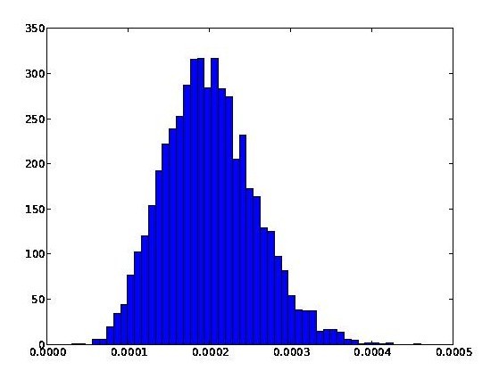
We see from this graph that PageRank has a mean of [tex]1/5000[/tex], as we expect, and an empirical standard deviation of [tex]0.000055[/tex]. Roughly speaking, it looks Gaussian, although, of course, PageRank is bounded above and below, and so can’t literally be Gaussian.

Suppose now that we change the number of links per page to [tex]100[/tex], but keep everything else the same. Then the resulting histogram is:

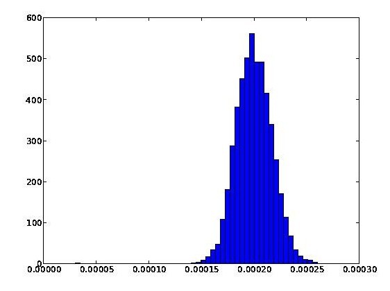
This also looks Gaussian, but has a smaller standard deviation of [tex]0.000017[/tex]. Notice that while we approach the minimal possible value of PageRank ([tex]t/N = 0.00003[/tex]) in the first graph, in neither graph do we come anywhere near the maximal possible value of PageRank, which is just a tad over [tex]s = 0.85[/tex].

Looking at these results, and running more numerical experiments in a similar vein, we see that as the number of outgoing links is increased, the standard deviation in PageRank seems to decrease. A bit of playing around suggests that the standard deviation decreases as one over the square root of the number of outgoing links, at least when the number of outgoing links is small compared with the total number of pages. More numerical experimentation suggests that the standard deviation is also proportional to [tex]s/N[/tex]. As a result, I conjecture:

Conjecture: Consider a random web with [tex]n[/tex] pages and [tex]m[/tex] outgoing links per page. Then for [tex]1 \ll m \ll n[/tex] the PageRank distribution approaches a Gaussian with mean [tex]1/n[/tex] and standard deviation [tex]s/(n\sqrt{m})[/tex].

For the case [tex]n = 5000, m = 10, s = 0.85[/tex] this suggests a standard deviation of [tex]0.000054[/tex], while for the case [tex]n = 5000, m = 100, s = 0.85[/tex] it suggests a standard deviation of [tex]0.000017[/tex]. Both these results are in close accord with the earlier empirical findings. The further numerical investigations I’ve done (not a lot, it must be said) also confirm it.

Incidentally, you might wonder why I chose to use a web containing [tex]5,000[/tex] pages. The way I’ve computed PageRank in the program above, we compute the matrix inverse of a [tex]5,000[/tex] by [tex]5,000[/tex] matrix. Assuming we’re using [tex]64[/tex]-bit floating point arithmetic, that means just storing the matrix requires [tex]200[/tex] megabytes. Not surprisingly, it turns out that my small laptop can’t cope with [tex]10,000[/tex] webpages, so I stuck with [tex]5,000[/tex]. Still, it’s notable that at that size the program still ran quite quickly. In the next lecture we’ll see how to cope with much larger sets of webpages.

Exercises

• Modify the program above to run with [tex]m=1[/tex]. You’ll find that the PageRank distribution does not look Gaussian. What conjecture do you think describes the PageRank distribution in this case? What’s a good reason we might not expect Gaussian behaviour for small values of [tex]m[/tex]?
• Do you trust the Python code to produce the correct outcomes? One of the problems in using numeric libraries as black boxes is that it can be hard to distinguish between real results and numerical artifacts. How would you determine which is the case for the code above? (For the record, I do believe the results, but have plans to do more checks in later lectures!)

Problems

• Can you prove or disprove the above conjecture? If it’s wrong, is there another similar type of result you can prove for PageRank, a sort of “central limit theorem” for PageRank? Certainly, the empirical results strongly suggest that some type of result in this vein is true! I expect that a good strategy for attacking this problem is to first think about the problem from first principles, and, if you’re getting stuck, to consult some of the literature about random walks on random graphs.
• What happens if instead of linking to a fixed number of webpages, the random link structure is governed by a probability distribution? You might like to do some computational experiments, and perhaps formulate (and, ideally, prove) a conjecture for this case.
• Following up on the last problem, I believe that a much better model of the web than the one we’ve used is to assume a power-law distribution of incoming (not outgoing) links to every page. Can you formulate (and, ideally, prove) a type of central limit theorem for PageRank in this case? I expect to see a much broader distribution of PageRanks than the Gaussian we saw in the case of a fixed number of outgoing links.

A simple technique to spam PageRank

One of the difficulties faced by search engines is spammers who try to artificially inflate the prominence of webpages by pumping up their PageRank. To defeat this problem, we need to understand how such inflation can be done, and find ways of avoiding it. Here’s one simple technique for getting a high PageRank.

Suppose the web contains [tex]N[/tex] pages, and we build a link farm containing [tex]M[/tex] additional pages, in the star topology described earlier. That is, we number our link farm pages [tex]1,\ldots,M[/tex], make page [tex]1[/tex] link only to itself, and all the other pages link only to page [tex]1[/tex]. Then if we use the original PageRank, with uniform teleportation probabilities [tex]1/(N+M)[/tex], a similar argument to earlier shows that the PageRank for page [tex]1[/tex] is

[tex] (s + t/M) \frac{M}{M+N}. [/tex]

As we increase the size, [tex]M[/tex], of the link farm it eventually becomes comparable to the size of the rest of the web, [tex]N[/tex], and this results in an enormous PageRank for page [tex]1[/tex] of the link farm. This is not just a theoretical scenario. In the past, spammers have built link farms containing billions of pages, using a technique similar to that described above to inflate their PageRank. They can then sell links from page 1 to other pages on the web, essentially renting out some of their PageRank.

How could we defeat this strategy? If we assume that we can detect the link farm being built, then a straightforward way of dealing with it is to modify the teleportation vector so that all pages in the link farm are assigned teleportation probabilities of zero, eliminating all the spurious PageRank accumulated due to the large number of pages in the link farm. Unfortunately, this still leaves the problem of detecting the link farm to begin with. That’s not so easy, and I won’t discuss it in this lecture, although I hope to come back to it in a later lecture.

Exercises

• Prove that the PageRank for page [tex]1[/tex] of the link farm is, as claimed above, [tex](s+t/M) M/(M+N)[/tex].
• The link topology described for the link farm is not very realistic. To get all the pages into the Google index the link farm would need to be crawled by Google’s webcrawler. But the crawler would never discover most of the pages, since they aren’t linked to by any other pages. Can you think of a more easily discoverable link farm topology that still gains at least one of the pages a large PageRank?

That concludes the second lecture. Next lecture, we’ll look at how to build a more serious implementation of PageRank, one that can be applied to a web containing millions of pages, not just thousands of pages.